About two months ago there was new SaaS product, the Keyword Hero. It’s the only solution to “decrypt” the organic keywords in Google Analytics that users searched for in order to get to one’s website. We do so by buying lots of data off sources such as plugins and matching the data with our customers’ sessions in Google Analytics (side note: the entire algorithm was coded in R before we refactored it in Python to allow scalability and operability with AWS).
Using Keyword Planner to evaluate markets
In order to assess the global potential of the tool and develop a market entry and distribution strategy, we used Google’s Keyword Planner.
The tool is widely used to get an initial understanding of market size and customer acquisition cost, as one sees the search volume (a proxy for market size) the average cost per click (a proxy for customer acquisition cost).
[This post is not about developing the right roll out strategy but about gathering valuable data for it in an efficient manner.]
Disappointing results for international research
Google offers some insights into keywords across countries: e.g. if you’d like to find out how the search volume for “python” varies among countries, you’ll get this:
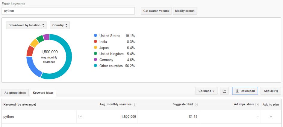
But what you get is a disappointment: almost 60% of the search volume is aggregated as “other countries”, you only get a very rough idea about the size, and no idea about the costs per click.
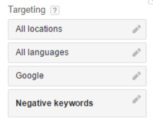
Way too little for anyone to work with and a far cry from what you’d get if you looked at the countries individually by using these targeting options:
Getting the real deal!
Google offers an API to retrieve the data. However, there are two problems with the API:
1. To use it, you need to apply for a Google AdWords’ developer token.
2. RAdwords doesn’t support the API, so you’d have to code the authentication and the queries without using RAdwords’ packages.
So we opted for the easier solution and decided to crawl the data with RSelenium:
Crawling Google’s Keyword Planner with RSelenium in 8 steps:
Google’s HTML is well structured, which makes querying fairly easy:
1. Start RSelenium
library(RSelenium)
driver<- rsDriver(browser = c(“firefox”))
remDr <- driver[[“client”]]
#navigate to AdWords-keywordplanner
remDr$navigate(“https://adwords.google.com/ko/KeywordPlanner/Home”)
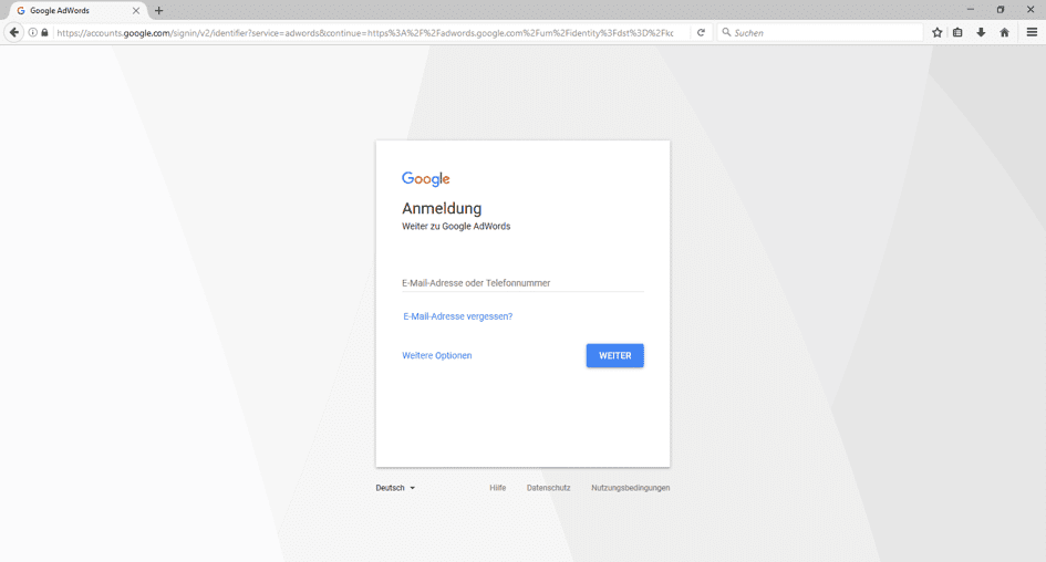
2. Sign in to AdWords manually
As the sign-in only needs to be done once, we didn’t write any code or this but did it manually.
3. Choose a set of keywords
Come up with a set of all keywords that help you assess your market.
In some verticals, such as SEO this is rather simple, as the lingua franca of SEOs and web analysts is English. For other products or services, you might have to use a set of keywords in multiple languages to generate meaningful and comparable data.
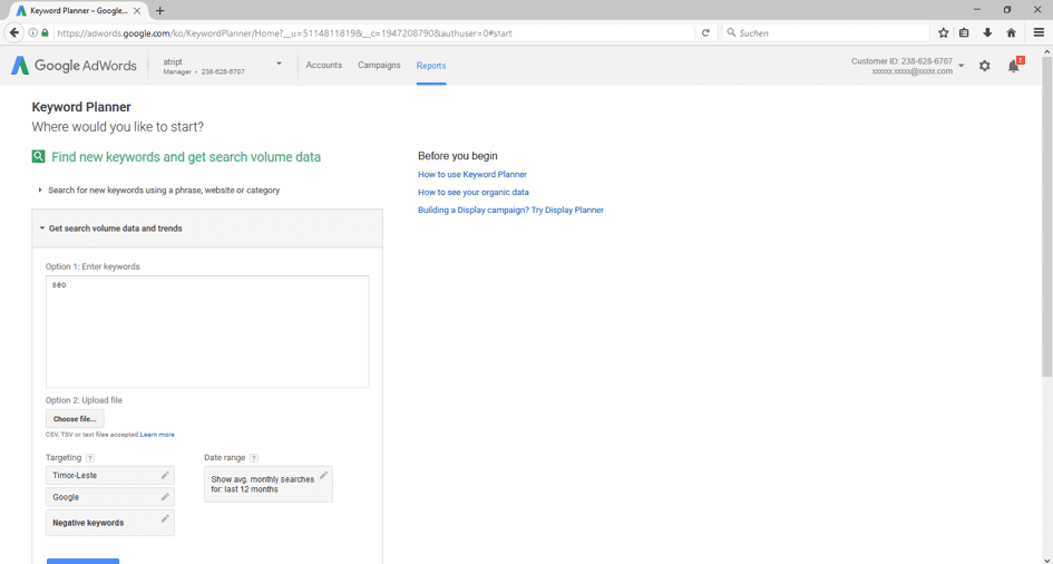
We enter the keyword we’d like to analyze at “Get search volume data and trends”. You can enter up to 3000 keywords (if you plan on using >100 keywords, make RSelenium save the data as .csv first), we used a set of about 30 keywords.
4. Import the regions you’d like to query
Before you can start crawling, you need a list of all regions (cities, countries, regions) that you’d like to generate data about. We pulled a list of all countries off Wikipedia and imported it to R:
#Import list of countries
library(readr)
countries<- read_csv(“C:/Users/User/Downloads/world-countries.csv”)
5. Query the first keywords without region manually
To get to the right URL, you need to query AdWords manually once, using your keyword set and without choosing any region at all.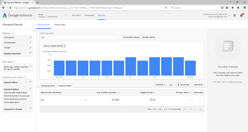
6. Start the loop
Now start the loop, that will insert the regions, query AdWords and save the results:
for (i in 1:nrow(countries)){
#Navigate to Data
#click on locations
css<-“.spMb-z > div:nth-child(1) > div:nth-child(3) > div:nth-child(2)”
x<-try(remDr$findElement(using=’css selector’,css))
x$clickElement()
#delete current locations
current_loc<-“#gwt-debug-positive-targets-table > table:nth-child(1) > tbody:nth-child(2) > tr:nth-child(1) > td:nth-child(3) > a:nth-child(1)”
x<-try(remDr$findElement(using=’css selector’,current_loc))
x$clickElement()
#click to insert text
css<-“#gwt-debug-geo-search-box”
x<-try(remDr$findElement(using=’css selector’,css))
#insert some stuff to be able to add data
x$sendKeysToElement(list(“somestuff”))
x$clearElement()
y<-as.character(countries[i,])
x$sendKeysToElement(list(y))
Sys.sleep(5)
#take the first hit
first_hit<-“.aw-geopickerv2-bin-target-name”
x<-try(remDr$findElement(using=’css selector’,first_hit))
x$clickElement()
#click save
save<-“.sps-m > div:nth-child(2) > div:nth-child(1) > div:nth-child(1) > div:nth-child(2)”
x<-try(remDr$findElement(using=’css selector’,save))
x$clickElement()
#Save the data
Sys.sleep(5)
#get the searchvolume
avgsv<-“#gwt-debug-column-SEARCH_VOLUME_PRIMARY-row-0-0”
x<-try(remDr$findElement(using=’css selector’,avgsv))
searchvolume[[i]]<-x$getElementText()
#get the bids
cpc<-“#gwt-debug-column-SUGGESTED_BID-row-0-1”
x<-try(remDr$findElement(using=’css selector’,cpc))
sug_cpc[[i]]<-x$getElementText()
}
7. Clean the data set
#clear the dataset
c<-as.data.frame(sug_cpc)
c<-t(c)
euro <- “\u20AC”
c<-gsub(euro,””,c)
c<-as.data.frame(as.numeric(c))
s<-as.data.frame(searchvolume)
s<-t(s)
s<-gsub(“,”,””,s)
s<-as.numeric(s)
#bind the data
all_countrys<-cbind(countries, s, c)
#clear the data from small countrys and wrong data (some small countrys don´t make really sense, so we eliminate them)
all_countrys<-sqldf(“SELECT * from all_countrys where s <200000 and c<30”)
#countrys as UTF-8
all_countrys$country<- stri_encode(all_countrys$country, “”, “UTF-8”)
8. Plot the data
#Plot with plotly
librayr(plotly)
a <- list(title = “search volume”)
b <- list(title = “costs”)
our_plot<-plot_ly(all_countrys, x=~s, y=~c, text=~country) %>%
layout(xaxis = a, yaxis = b, showlegend = FALSE)
#show_plot and view data
our_plot
View(all_countrys)
Evaluating the results of our set of SEO keywords
On the X-axis you see the costs per click, on the Y axis the search volume per country.
The US market strongly dominates the volume for SEO related keywords and is far off on the right. Note that the US is also pretty far up the top, which means high marketing expenses per user.
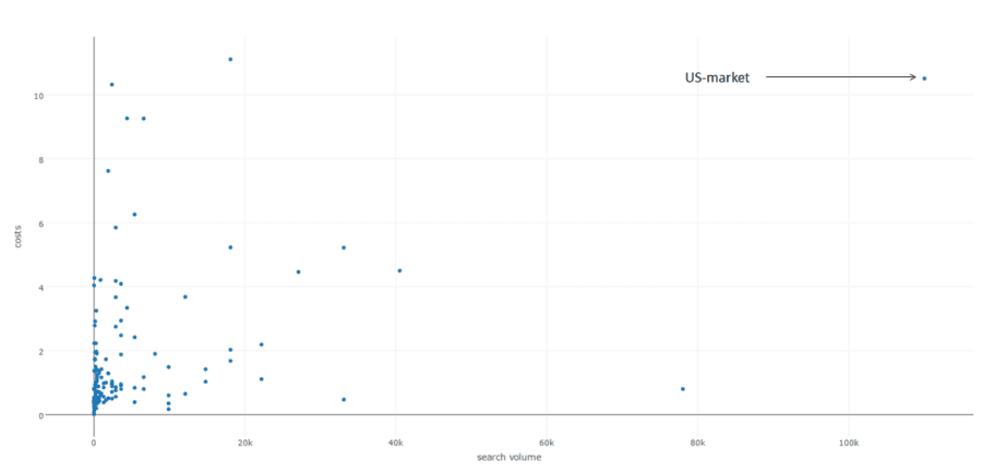
As a start-up, we’re looking for a large yet less competitive market for our paid ads (and focus on less costly marketing strategies in the US). So we ignore the US and adjust our plot a bit:
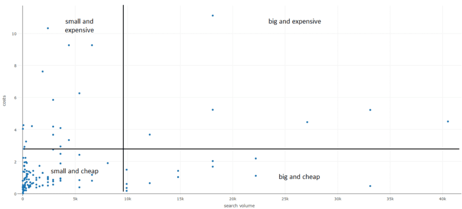
We segment the markets into four: “small and cheap”, “small and expensive”, “big and expensive” and “big and cheap”.
As we’re constrained by limited funds, we focus on the cheap markets (bottom) and ignore the expensive ones (top). As the initial effort to set up a marketing campaign is the same for a “small and cheap” (left) and a “big and cheap” (right) region, we naturally opt for the big ones (bottom right).
According to the data, the cheapest yet sizable markets to penetrate are countries such as Turkey, Brasil, Spain, Italy, France, India, and Poland. There is significant search volume (=interest) about SEO related topics and low costs per click (=little competition), which – in theory – should make market penetration fairly cheap and easy.
Obviously, this is quite a simplistic model but it provides a nice foundation for further thoughts. In a future blog post, we will check whether the correlation between this data and reality (= our efforts) is significant at all.
Here is the entire R code in one piece again:
#Crawl AdWords-keywordplanner by Country
library(RSelenium)
library(readr)
library(stringi)
library(sqldf)
library(plotly)
driver<- rsDriver(browser = c(“firefox”))
remDr <- driver[[“client”]]
#navigate to AdWords-keywordplanner
remDr$navigate(“https://adwords.google.com/ko/KeywordPlanner/Home”)
#Import csv with countrys
countries<- read_csv(“C:/Users/User/Downloads/laender_der_welt.csv”)
for (i in 1:nrow(countries)){
#Navigate to Data
#click on locations
css<-“.spMb-z > div:nth-child(1) > div:nth-child(3) > div:nth-child(2)”
x<-try(remDr$findElement(using=’css selector’,css))
x$clickElement()
#delete current locations
current_loc<-“#gwt-debug-positive-targets-table > table:nth-child(1) > tbody:nth-child(2) > tr:nth-child(1) > td:nth-child(3) > a:nth-child(1)”
x<-try(remDr$findElement(using=’css selector’,current_loc))
x$clickElement()
#click to insert text
css<-“#gwt-debug-geo-search-box”
x<-try(remDr$findElement(using=’css selector’,css))
#insert some stuff to be able to add data
x$sendKeysToElement(list(“somestuff”))
x$clearElement()
y<-as.character(countries[i,])
x$sendKeysToElement(list(y))
Sys.sleep(5)
#take the first hit
first_hit<-“.aw-geopickerv2-bin-target-name”
x<-try(remDr$findElement(using=’css selector’,first_hit))
x$clickElement()
#click save
save<-“.sps-m > div:nth-child(2) > div:nth-child(1) > div:nth-child(1) > div:nth-child(2)”
x<-try(remDr$findElement(using=’css selector’,save))
x$clickElement()
#Save the data
Sys.sleep(5)
#get the searchvolume
avgsv<-“#gwt-debug-column-SEARCH_VOLUME_PRIMARY-row-0-0”
x<-try(remDr$findElement(using=’css selector’,avgsv))
searchvolume[[i]]<-x$getElementText()
#get the bids
cpc<-“#gwt-debug-column-SUGGESTED_BID-row-0-1”
x<-try(remDr$findElement(using=’css selector’,cpc))
sug_cpc[[i]]<-x$getElementText()
}
#clear the dataset
c<-as.data.frame(sug_cpc)
c<-t(c)
euro <- “\u20AC”
c<-gsub(euro,””,c)
c<-as.data.frame(as.numeric(c))
s<-as.data.frame(searchvolume)
s<-t(s)
s<-gsub(“,”,””,s)
s<-as.numeric(s)
#bind the data
all_countrys<-cbind(countries, s, c)
#clear the data from small countrys and wrong data (some small countrys don´t make really sense, so we eliminate them)
all_countrys<-sqldf(“SELECT * from all_countrys where s <200000 and c<30”)
#countrys as UTF-8
all_countrys$country<- stri_encode(all_countrys$country, “”, “UTF-8”)
#Plot with plotly
a <- list(title = “search volume”)
b <- list(title = “costs”)
q<-plot_ly(all_countrys, x=~s, y=~c, text=~country) %>%
layout(xaxis = a, yaxis = b, showlegend = FALSE)
#show_plot and view data
q
View(all_countrys)
