Using Confusion Matrices to Quantify the Cost of Being Wrong

There are so many confusing and sometimes even counter-intuitive concepts in statistics.  I mean, come on…even explaining the differences between Null Hypothesis and Alternative Hypothesis can be an ordeal.  All I want to do is to understand and quantify the cost of my analytical models being wrong.

For example, let’s say that I’m a shepherd who has bad eyesight and have a hard time distinguishing between a wolf and a sheep dog.  That’s obviously a bad trait, because the costs of being wrong are very expensive:

• There are times when I confuse a wolf for a sheep dog and take no action, which results in loss of sheep. The incident costs me $2,000 per occurrence and happens 10% of the time.
• Alternatively, there are times when I confuse a sheep dog for a wolf and accidently kill the sheep dog, which results in the flock being unprotected. The incident costs me $5,000 per occurrence and happens 5% of the time.

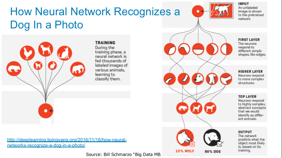
Okay, so I’m not a very good shepherd, but I am a very sophisticated shepherd and I’ve build a Neural Network application to distinguish a sheep dog from a wolf.  Through much training of the “Wolf Detection” neural network, I now have a tool that can correctly distinguish a sheep dog from a wolf with 95% accuracy (see Figure 1).

Figure 1: Source: “Why Deep Learning Is Suddenly Changing Your Life” http://fortune.com/ai-artificial-intelligence-deep-machine-learning…

Okay, that seems pretty great, but is 95% accuracy good enoughgiven the costs of False Positives and False Negatives? Shouldn’t I invest more time and effort to improve that accuracy percentage to ensure that my model is “profitable;” quantify that 5% inaccuracy which is making my analytical model wrong?

Enter the Confusion Matrix (if there was ever an accurate description of something, this name nails it).

Understanding the Confusion Matrix

So how does one go about quantifying the costs of being wrong using the Confusion Matrix? That is, determining if a model that correctly predicts with, for instance, 95% accuracy is good enough given the business situation and the costs associated with being wrong. 

The terms ‘true condition’ (‘positive outcome’) and ‘predicted condition’ (‘negative outcome’) are used when discussing Confusion Matrices.  This means that you need to understand the differences (and eventually the costs associated) with Type I and Type II Errors.

• Type I Error (or False Positive) is a result that indicates that a given condition is present when it actually is not present. In our shepherd example, that would be incorrectly identifying the animal as a wolf when in reality it is a dog.
• Type II Error (or False Negative) is a result that indicates that a given condition is not present when it actually is present.  In our shepherd example, that would be incorrectly identifying the animal as a dog when in reality it is a wolf.

First, let’s set up our Confusion Matrix for testing the condition: “Is that animal in the grove a wolf?” The Positive Condition is “The Animal is a Wolf” in which case I’d take the appropriate action (probably wouldn’t try to pet it).  Below is the 2×2 Confusion Matrix for our use case.

Where:

• True Positive (TP) where the True Condition was wolf and the model accurately predicted a wolf.
• True Negative (TN) where the True Condition was a dog and the model accurately predicted a dog.
• False Positive (FP) which is a Type I Error where the True Condition was a dog and the model inaccurately predicted a wolf (so that I accidently shoot the dog protecting the sheep).
• False Negative (FN) which is a Type II Error where the True Condition is a wolf but the model inaccurately predicted a dog (so that I ignore the wolf and it feasts on the sheep smorgasbord).

So once the neural network model produces the Confusion Model that covers all four of the above conditions in the 2×2 matrix, we can calculate goodness of fit and effectiveness measures, such as model Precision, Sensitivity and Specificity.

The Confusion Matrix can then be used to create the following measures of goodness of fit and model accuracy.

• Precision = TP / (TP + FP)
• Recall or Sensitivity = TP / (TP + FN)
• Specificity = TN / (FP + TN)
• Accuracy = (TP + TN) / (TP + FP + TN + FN)

Putting the Confusion Matrix to Work

Now let’s get back to our shepherd example.  We want to determine the costs of the model being wrong, or the savings the neural network provides.  We need to determine if the there is sufficient improvement in what the model provides over what the shepherd already does himself.

Before the Wolf Detection application, I (as the shepherd) had the following Confusion Matrix where:

• False Positives10% of the time, where he mistakes a wolf for a sheep dog, took no action, and the wolf causes $2,000 of damage.
• False Negatives 5% of the time, where he mistakes a sheep dog for a wolf, accidently kill the sheep dog and leaves the flock unprotected which $5,000 of damage.

By the previous definitions, the corresponding metrics without using the Wolf Detection Application are:

• Precision = 88%
• Recall / Sensitivity = 94%
• Specificity = 50%
• Accuracy = 85%

Now using the Wolf Detection application, we get the below Confusion Matrix:

Confusion Matrix metrics with using the Wolf Detection Application are:

• Precision = 95%
• Recall/Sensitivity = 99%
• Specificity = 79%
• Accuracy = 95%

Bringing this all together into a single table:

Return on Investment then equals:

• Reduction in False Positives from 10% to 4% (which saves $2,000 per occurrence)
• Reduction in False Negatives from 5% to 1% (which saves $5,000 per occurrence)

Finally, the Expected Value Per Prediction (EvP) =

= ($2000 * Change in FP%) + ($5000 * Change in FN%)

= ($2000*.06) + ($5000*.04)

= $320 average savings per night

Summary

Not all Type I and Type II errors are of equal value.  One needs to invest the time to understand the costs of Type I and Type II errors in relationship to your specific case.  The real challenge is determining whether the improvement in performance from the analytic model is “good enough.”  The Confusion Matrix can help us make that determination.

And if folks are still struggling with the concept of Type I and Type II errors, I hope the below image can help to clarify the difference.  Hehehe

Special thanks to Larry Berk, one of my Senior Data Scientists, for his guidance on this blog. He still understands the use of Confusion Matrices much better than me!

Sources:

“Simple Guide to Confusion Matrix Terminology”

“Confusion Matrix” from Wikipedia (by the way, I did make a donation to Wikipedia. They are a valuable source of information for these sorts of topics).