In this article, we shall see how the Bayesian Kalman Filter can be used to predict positions of some moving particles / objects in 2D.
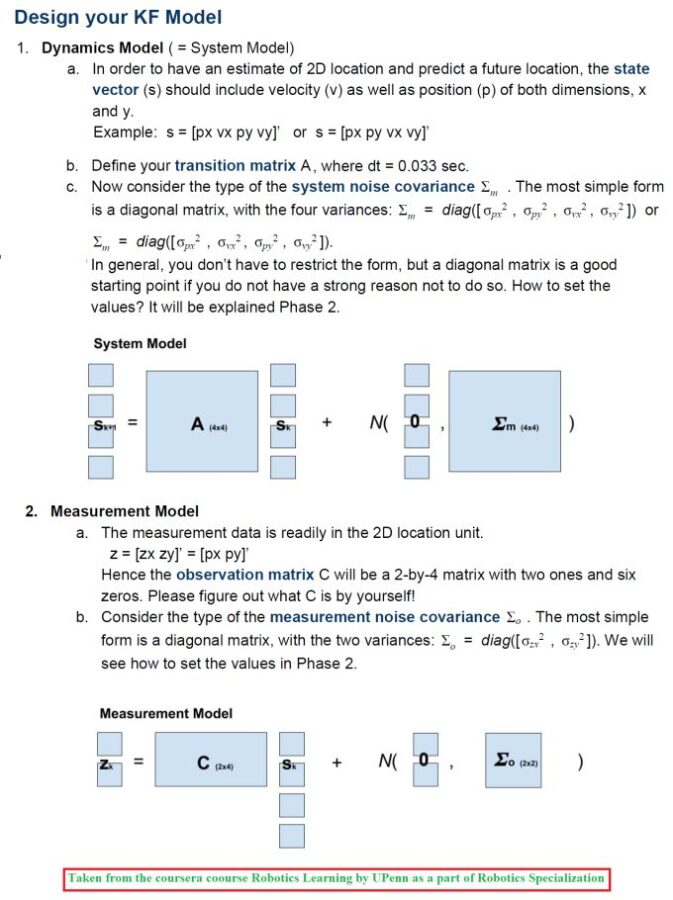
This article is inspired by a programming assignment from the coursera course Robotics Learning by University of Pennsylvania, where the goal was to implement a Kalman filter for ball tracking in 2D space. Some part of the problem description is taken from the assignment description.
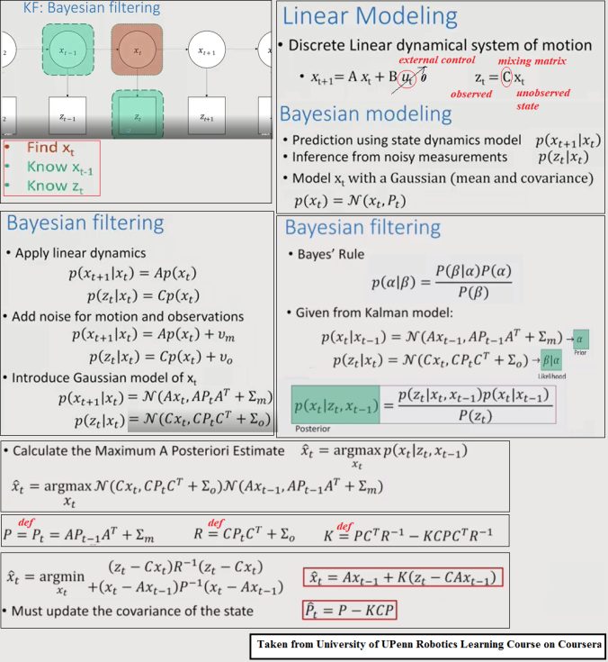
The following equations / algorithms are going to be used to compute the Bayesian state updates for the Kalman Filter.
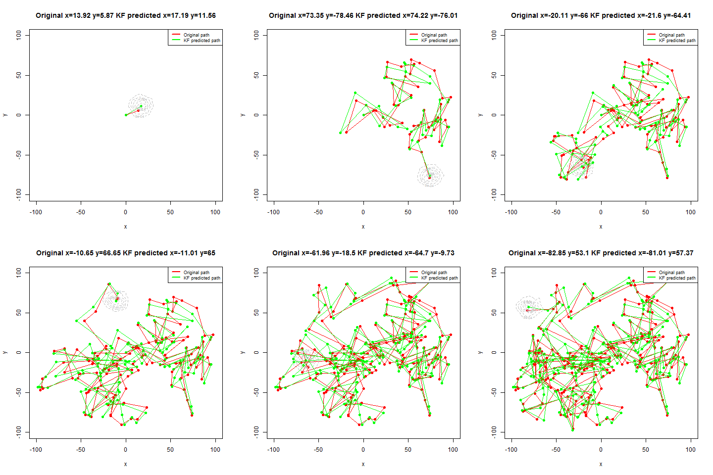
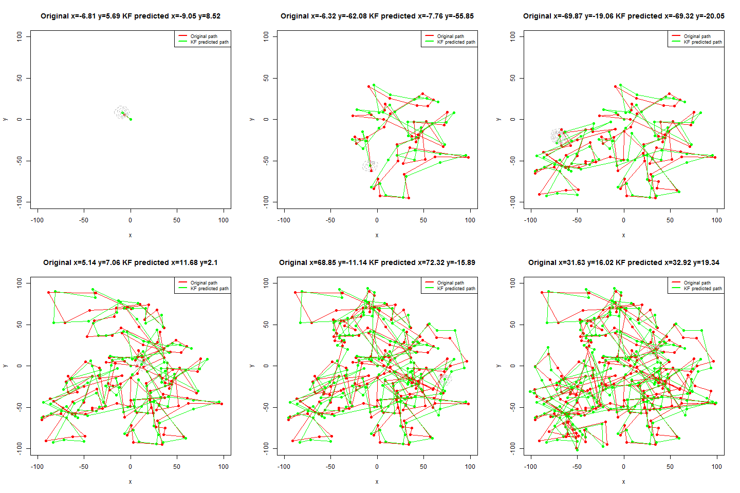
For the first set of experiments, a few 2D Brownian Motion like movements are simulated for a particle.
- The noisy position measurements of the particle are captured at different time instants (by adding random Gaussian noise).
- Next, Kalman Filter is used to predict the particle’s position at different time instants, assuming different position, velocity and measurement uncertainty parameter values.
- Both the actual trajectory and KF-predicted trajectory of the particle are shown in the following figures / animations.
- The positional uncertainty (as 2D-Gaussian distribution) assumed by the Kalman Filter is also shown as gray / black contour (for different values of uncertainties).


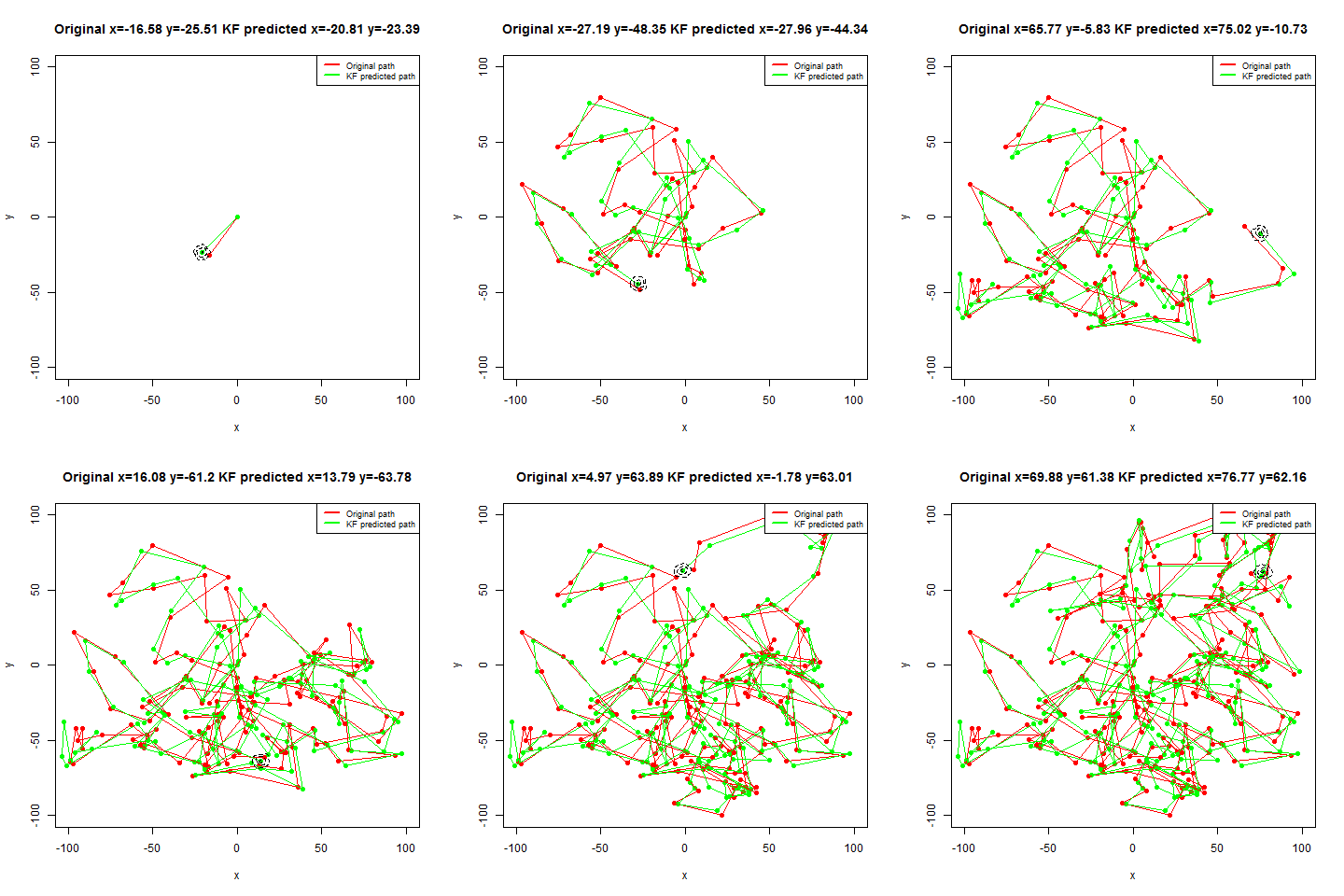
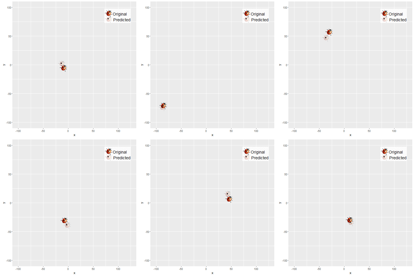
The next set of figures / animations show how the position of a moving bug is tracked using Kalman Filter.
- First the noisy measurements of the positions of the bug are obtained at different time instants.
- Next the correction steps and then the prediction steps are applied, after assuming some uncertainties in position, velocity and the measurements with some Gaussian distributions.

- The position of the bug as shown in the figure above is moving in the x and ydirection randomly in a grid defined by the rectangle [-100,100]x[-100,100].
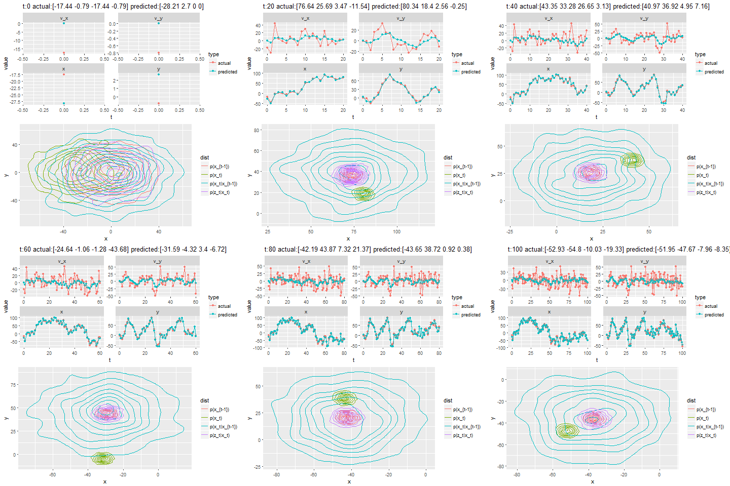
- The next figure shows how different iterations for the Kalman Filter predicts and corrects the noisy position observations. The uncertain motion model p(x_t|x_{t-1}) increases the spread of the contour. We observe a noisy position estimate z_t. The contour of the corrected position p(x_t) has less spread than both the observation p(z_t|x_t) and the motion p(x_t|x_{t-1}) adjusted state.
-

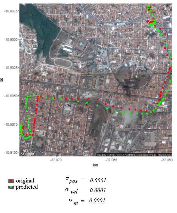
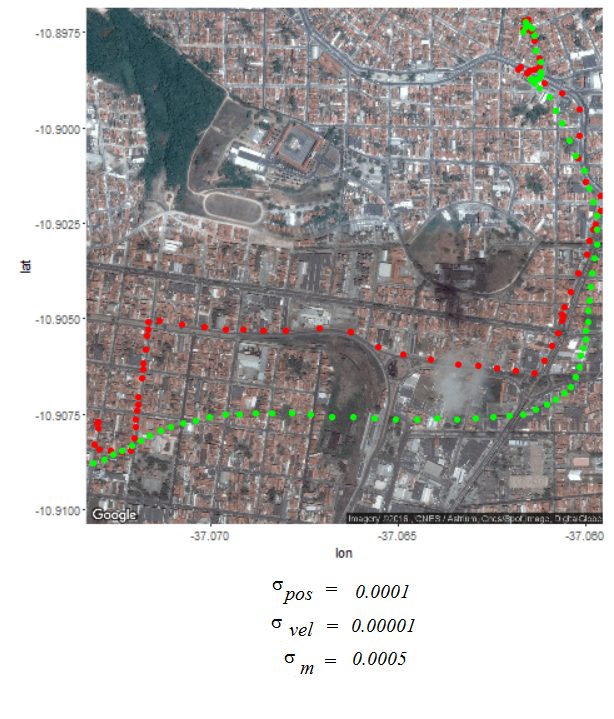
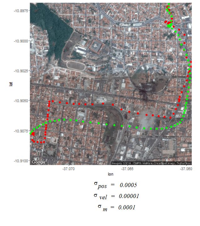
Next the GPS dataset from the UCI Machine Learning Repository is used to get the geospatial positions of some vehicles at different times.
- Again some noisy measurement is simulated by adding random noise to the original data.
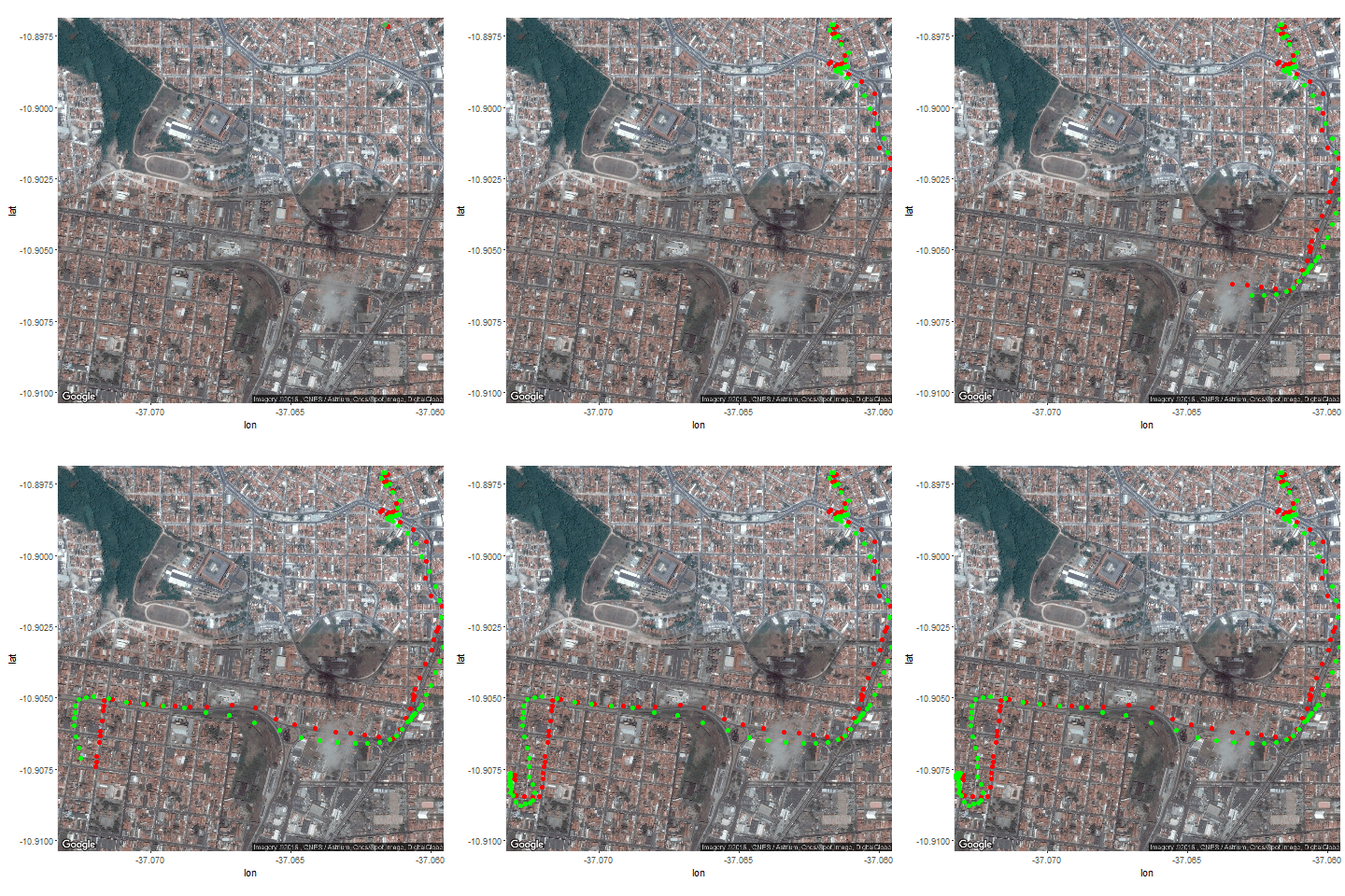
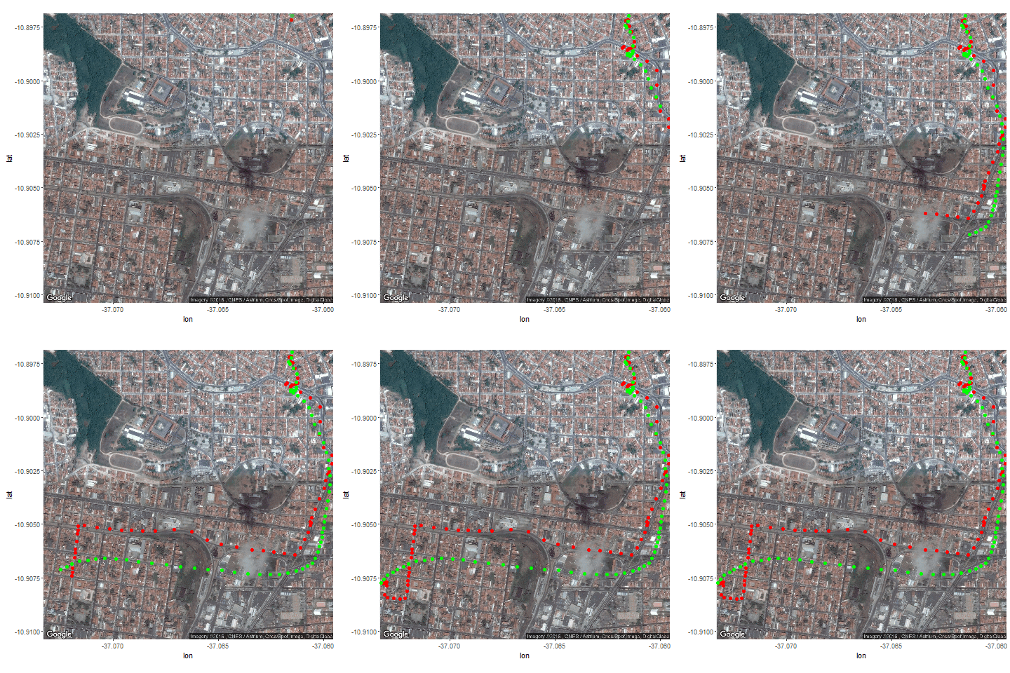
- Then the Kalman Filter is again used to predict the vehicle’s position at different time instants, assuming different position, velocity and measurement uncertainties.
- The position and measurement uncertainties (σ_p, σ_m) are in terms of latitude / longitude values, where uncertainty in the motion model is σ_v.
- Both the actual trajectory and KF-predicted trajectory of the vehicle are shown in the following figures / animations.
- As expected, the more the uncertainties in the position / motion model, the more the actual trajectory differs from the KF-predicted one.


