This article comes from Algobeans Layman tutorials in analytics.
Whenever you spot a trend plotted against time, you would be looking at a time series. The de facto choice for studying financial market performance and weather forecasts, time series are one of the most pervasive analysis techniques because of its inextricable relation to time—we are always interested to foretell the future.
Temporal Dependent Models
One intuitive way to make forecasts would be to refer to recent time points. Today’s stock prices would likely be more similar to yesterday’s prices than those from five years ago. Hence, we would give more weight to recent than to older prices in predicting today’s price. These correlations between past and present values demonstrate temporal dependence, which forms the basis of a popular time series analysis technique called ARIMA (Autoregressive Integrated Moving Average). ARIMA accounts for both seasonal variability and one-off ‘shocks’ in the past to make future predictions.
However, ARIMA makes rigid assumptions. To use ARIMA, trends should have regular periods, as well as constant mean and variance. If, for instance, we would like to analyze an increasing trend, we have to first apply a transformation to the trend so that it is no longer increasing but stationary. Moreover, ARIMA cannot work if we have missing data.
To avoid having to squeeze our data into a mould, we could consider an alternative such as neural networks. Long short-term memory (LSTM) networks are a type of neural networks that builds models based on temporal dependence. While highly accurate, neural networks suffer from a lack of interpretability—it is difficult to identify the model components that lead to specific predictions.
General Additive Modela
Besides using correlations between values from similar time points, we could take a step back to model overall trends. A time series could be seen as a summation of individual trends. Take, for instance, google search trends for persimmons, a type of fruit.
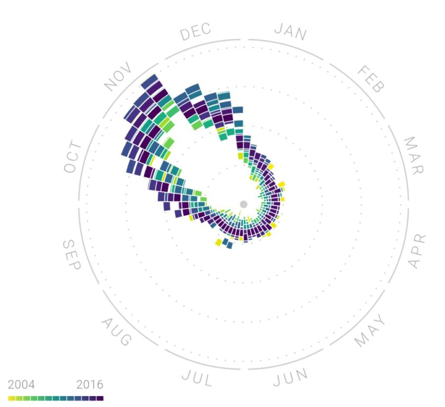
From the Figure 1, we can infer that persimmons are probably seasonal. With its supply peaking in November, grocery shoppers might be prompted to google for nutrition facts or recipes for persimmons.

Figure 1. Seasonal trend in google searches for ‘persimmon’ (source: click here)
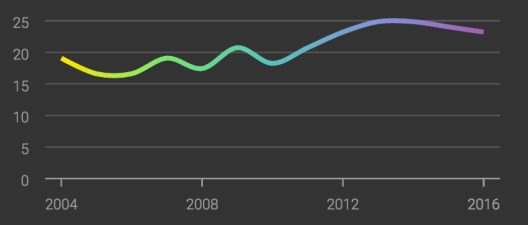
Moreover, google searches for persimmons are also growing more frequent over the years.

Figure 2. Overall growth trend in google searches for ‘persimmon’ (source:click here)
Therefore, google search trends for persimmons could well be modeled by adding a seasonal trend to an increasing growth trend, in what’s called a generalized additive model (GAM).
The principle behind GAMs is similar to that of regression, except that instead of summing effects of individual predictors, GAMs are a sum of smooth functions. Functions allow us to model more complex patterns, and they can be averaged to obtain smoothed curves that are more generalizable.
Because GAMs are based on functions rather than variables, they are not restricted by the linearity assumption in regression that requires predictor and outcome variables to move in a straight line. Furthermore, unlike in neural networks, we can isolate and study effects of individual functions in a GAM on resulting predictions.
In this tutorial, you will:
- See an example of how GAM is used.
- Learn how functions in a GAM are identified through backfitting.
- Learn how to validate a time series model.
To check out all this information, click here.
DSC Resources
- Services: Hire a Data Scientist | Search DSC | Classifieds | Find a Job
- Contributors: Post a Blog | Ask a Question
- Follow us: @DataScienceCtrl | @AnalyticBridge
Popular Articles
