Understanding the maths behind forward and back propagation is not very easy.
There are some very good – but also very technical explanations.
For example : The Matrix Calculus You Need For Deep Learning Terence Parr and Jer…is an excellent resource but still too complex for beginners.
I found a much simpler explanation in the ml cheatsheet.
The section below is based on this source.
I have tried to simplify this explanation as below.
All diagrams and equations are based on this source in the ml cheatsheet
Forward propagation

Let’s start with forward propagation
Here, input data is “forward propagated” through the network layer by layer to the final layer which outputs a prediction. The simple network can be seen as a series of nested functions.
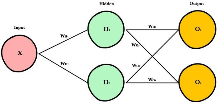
For the neural network above, a single pass of forward propagation translates mathematically to:
A ( A( X Wh) Wo )
Where
A is an activation function like ReLU,
X is the input
Wh and Wo are weights for the hidden layer and output layer respectively
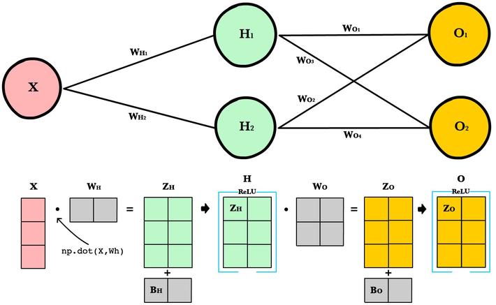
A more complex network can be shown as below

INPUT_LAYER_SIZE = 1
HIDDEN_LAYER_SIZE = 2
OUTPUT_LAYER_SIZE = 2
In matrix form, this is represented as:

|
Var |
Name |
Dimensions |
|
X |
Input |
(3, 1) |
|
Wh |
Hidden weights |
(1, 2) |
|
Bh |
Hidden bias |
(1, 2) |
|
Zh |
Hidden weighted input |
(1, 2) |
|
H |
Hidden activations |
(3, 2) |
|
Wo |
Output weights |
(2, 2) |
|
Bo |
Output bias |
(1, 2) |
|
Zo |
Output weighted input |
(3, 2) |
|
O |
Output activations |
(3, 2) |
Source: https://ml-cheatsheet.readthedocs.io/en/latest/forwardpropagation.html
Backpropagation
Now, let us explore backpropagation. In backpropagation, we adjust each weight in the network in proportion to how much it contributes to overall error. We iteratively reduce each weight’s error. Eventually, when the error is minimised, we have a series of weights the produce good predictions.
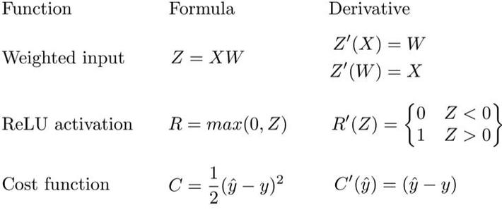
As we have seen before, forward propagation can be viewed as a series of nested functions. Hence, backpropagation can be seen as the application of the Chain rule to find the derivative of the cost with respect to any weight in the network. This represents how much each weight contributes to the overall error and the direction to update each weight to reduce the error. The error is then reduced through Gradient descent. The equations needed to make a prediction and calculate total error, or cost:

To use these equations:
- We first calculate the output layer error
- We pass this error back to the hidden layer before it
- At that hidden layer, we calculate the error (hidden layer error) pass the result to the hidden layer before it and so on.
- At every layer, we calculate the derivative of cost with respect that layer’s weights.
- This resulting derivative tells us in which direction to adjust our weights to reduce overall cost. This step is performed using Gradient descent algorithm.
Hence,
We first calculate the derivative of cost with respect to the output layer input, Zo. This gives us the impact of the final layer’s weights on the overall error in the network. The derivative is:
C′(Zo)=(y^−y)⋅R′(Zo)
Here
(y^−y) is the cost and
R′(Zo) represents the derivative of the ReLU activation for the output layer
This error is represented by Eo where
Eo=(y^−y)⋅R′(Zo)
Now, to calculate hidden layer error, we need to find the derivative of cost with respect to the hidden layer input, Zh. Following the same logic, this can be represented as
Eh=Eo⋅Wo⋅R′(Zh)
Where R′(Zh) represents the derivative of the Relu activation for the hidden layer
This formula is at the core of backpropagation.
- We calculate the current layer’s error
- Pass the weighted error back to the previous layer
- We continue the process through the hidden layers
- Along the way we update the weights using the derivative of cost with respect to each weight.
The Derivative of cost with respect to any weight is represented as
C′(w)=CurrentLayerError⋅CurrentLayerInput where Input refers to the activation from the previous layer, not the weighted input, Z.
Hence, the 3 equations that together form the foundation of backpropagation are

The process can be visualised as below:

These equations are not very easy to understand and I hope you find the simplified explanation useful
I keep trying to improve my own understanding and to explain them better
I welcome your comments
Source: adapted and simplified from the ml cheatsheet
