Let’s look at several techniques in machine learning and the math topics that are used in the process.
In linear regression, we try to find the best fit line or hyperplane for a given set of data points. We model the output of our linear function by a linear combination of the input variables using a set of parameters as weights.
The parameters are found by minimizing the residual sum of squares. We find a critical point by setting the vector of derivatives of the residual sum of squares to the zero vector. By the second derivative test, if the Hessian of the residual sum of squares at a critical point is positive definite, then the residual sum of squares has a local minimum there.
In the above process, we used derivatives, the second derivative test, and the Hessian, which are notions from multivariable calculus. We can also find the solution to our minimization problem using linear algebra.
Let X be the matrix where the rows are our data inputs, beginning with 1 in each row, and y be the vector of our data outputs. We want a vector β such that Xβ is close to y. In other words, we want a vector β such that the distance ‖Xβ-y‖ between Xβ and y is minimized. The vector β which minimizes the distance is such that Xβ is the projection of y onto the column space of X. This is so because the projection of y onto the column space of X is the vector in the column space of X that is closest to y. We then use the fact that Euclidean N-space can be broken into two subspaces, the column space of X and the orthogonal complement of the column space of X, and the fact that any vector in Euclidean N-space can be written uniquely as the sum of vectors in the column space of X and in the orthogonal complement of the column space of X, respectively, to deduce that y-Xβ is orthogonal to the columns of X. From here, we can arrive at the matrix equation X^T Xβ=X^T y. If X^T X is positive definite, then the eigenvalues of X^T X are all positive. So 0 is not an eigenvalue of X^T X. It follows that X^T X is invertible. Then, we can solve the matrix equation for β, and the result is the same result we get from using multi-variable calculus.
In the solution we just discussed, the notions of norm, projection, column space, subspace, orthogonal complement, orthogonality, positive definiteness, eigenvalue, and invertibility are used. These are notions from linear algebra. We also used the facts that Euclidean N-space can be broken into two subspaces, the column space of X and the orthogonal complement of the column space of X and that any vector in Euclidean N-space can be written uniquely as the sum of vectors in the column space of X and in the orthogonal complement of the column space of X, respectively.
Let’s turn to classification problems. In classification problems, we want to determine the class to which a data point belongs to. One of the methods used for classification problems is linear discriminant analysis.
In linear discriminant analysis, we estimate Pr(Y=k|X=x), the probability that Y is the class k given that the input variable X is x. This is called a posterior probability function. Once we have all of these probabilities for a fixed x, we pick the class k for which the probability Pr(Y=k|X=x) is largest. We then classify x as that class k.
Using Bayes’ rule, we can rewrite the posterior probability function in terms of π_k=Pr(Y=k), the prior probability that Y=k, and f_k (x)=Pr(X=x|Y=k), the probability that X=x, given that Y=k.
We assume that the conditional distribution of X given Y=k is the multivariate Gaussian distribution N(μ_k,Σ), where μ_k is a class-specific mean vector and Σ is the covariance of X. So f_k (x) can be rewritten in terms of μ_k and Σ.
Now, we find estimates for π_k,μ_k, and Σ, and hence for p_k (x). We classify x according to the class k for which the estimated p_k (x) is greatest.
In linear discriminant analysis, we use posterior probability functions, prior probabilities, Bayes’ rule, multivariate Gaussian distribution, class-specific mean vector, and covariance, which are notions from probability theory.
Another method for solving classification problems is logistic regression. Just as in linear discriminant analysis, we want to estimate Pr(Y=k|X=x) and pick the class k for which this probability is largest. Instead of estimating this probability indirectly using Bayes’ rule, as in linear discriminant analysis, we estimate the probability directly.
Assuming there are only two classes 0 and 1, let p(x)=Pr(Y=1|X=x). In logistic regression, we assume that the log-odds is a linear function of the components of x. Assuming that the log-odds is a linear function of the components of x, with parameters β_0,β_1,…,β_p, we can solve for p(x) as a function of the parameters and the components of x. We can get an estimate for p(x) if we had estimates for the parameters β_0,β_1,…,β_p.
The probability of our observed data is a function of the parameters β_0,β_1,…,β_p and is called a likelihood function. We find estimates for the parameters by maximizing the likelihood function. Maximizing the likelihood function is equivalent to maximizing the log of the likelihood function. To maximize the log-likelihood function, we use the Newton-Raphson method.
The log-likelihood function L(β) is a real-valued function of β=(β_0,β_1,…,β_p). So L is a function from R^(p+1) to R. Further, L is twice continuously differentiable. So we can apply the multivariate Newton-Raphson method.
In logistic regression, we use likelihood functions, a notion from probability theory, and the multivariate Newton-Raphson method, a notion from multivariable calculus.
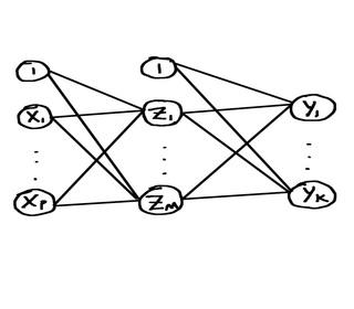
Next, we’ll look at a method that can be used to solve both regression and classification problems. In artificial neural networks, we use compositions of linear and nonlinear functions to model our output functions.
The output functions can be represented by a neural network diagram.

The input units, including the constant 1, will form the input layer. We take a linear combination of the input units, including the constant 1, and then apply an activation function h to it to get a new unit. h is a differentiable (possibly nonlinear) function. We do this, say, M times; we now have M hidden units, and these make up a hidden layer. Looking at the diagram, the weights in the linear combinations are represented by the line segments connecting two units. We can continue this process of taking linear combinations of the units in the previous layer and applying an activation function to each linear combination to create a new hidden unit and thus creating the next hidden layer. At some point we have a last layer, called the output layer, and we use activation functions g_k for each output unit Y_k. g_k is a function of all the linear combinations of the units from the previous layer.
Usually, the activation function h is chosen to be the logistic sigmoid function or the tanh function. The output activation functions g_k will differ depending on the type of problem, whether it’s a regression problem, a binary classification problem, or a multiclass classification problem.
So far, we’ve constructed output values Y_k that depend on an input x and that involve a bunch of unknown parameters. Our goal now is to use our training data to find values for the unknown parameters that minimize error. For binary classification, we find estimates for the parameters by maximizing the likelihood function associated with the probability of our observed data; this corresponds to minimizing what’s called the cross-entropy error function. Similarly, for multiclass classification, we find estimates for the parameters by maximizing the likelihood function associated with the probability of our observed data; this corresponds to minimizing what’s called the multiclass cross-entropy error function. For regression, we find estimates for the parameters by minimizing the sum-of-squares error function.
To minimize the error function, we use gradient descent, which requires finding the gradient of the error function. To find the gradient of the error function, we use backpropagation.
In artificial neural networks, the notion of likelihood function from probability theory is used in the case of classification problems. Gradient descent, from multivariable calculus, is used to minimize the error function. During backpropagation, the multivariable chain rule is used.
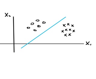
Let’s look at the method of support vector machines for solving classification problems. The idea is that we have a bunch of data points, say of two classes, and we want to separate them with a decision boundary. For instance, the data points might be easily separated by a line like this:

If the data points can be easily separated using a line or hyperplane, we find the separating hyperplane that is as far as possible from the points so that there is a large margin. This requires maximizing the margin, and it ends up being a convex optimization problem. To solve this convex optimization problem, we use Lagrange multipliers, a notion from multivariable calculus. Once we find the maximal margin hyperplane, we can classify new points depending on which side of the hyperplane the point lies on. This method of classifying points is called the maximal margin classifier.
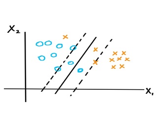
If the data points are not separable by a hyperplane, we can still try to find a hyperplane that separates most of the points but that may have some points that lie inside the margin or lie on the wrong side of the hyperplane. The situation may look like this:

Just as in the case of the maximal margin classifier, we want our hyperplane to be as far as possible from each point that’s on the correct side of the hyperplane. So points on the margin or outside the margin but on the correct side of the hyperplane will be as far as possible from the hyperplane. Points inside the margin but on the correct side of the hyperplane will be as far as possible from the hyperplane and as close as possible to the margin boundary. For those points on the wrong side of the hyperplane, we want those points to be as close to the hyperplane as possible.
Just as in the case of the maximal margin classifier, we want to maximize the margin so that points on the correct side of the hyperplane are as far as possible from the hyperplane.
Not only do we want to maximize the margin, we also want to minimize the violations of the margin. This problem turns out to be a convex optimization problem, and it is solved using Lagrange multipliers.
Once we find the separating hyperplane, called the soft margin hyperplane, we can classify new points depending on which side of the hyperplane the point lies on. This method of classifying points is called the soft margin classifier.
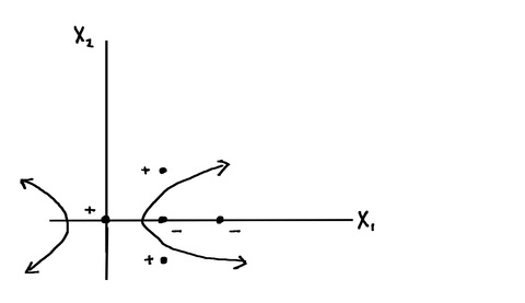
If the data points are not linearly separable and it appears that the decision boundary separating the two classes is non-linear, we can use what’s called the support vector machine, or support vector machine classifier. The idea is to consider a larger feature space with data points in this larger space associated with the original data points and to apply the support vector classifier to this new set of data points in the larger feature space. This will give us a linear decision boundary in the enlarged feature space but a non-linear decision boundary in the original feature space. Any new point is classified by sending it into the larger space and using the linear decision boundary. Here’s what a situation that requires support vector machines might look like:

In the process of solving the convex optimization problem for the soft margin classifier, a dot product occurs; in the method of support vector machines, we replace the dot product by something called a kernel. A kernel is essentially a function that can be represented as the inner product of the images of the input values under some transformation h. This replacement of the dot product with a kernel is called the kernel trick.
The kernel K should be a valid kernel; that is, there should be a feature space mapping h that corresponds to K. By Mercer’s theorem, it’s sufficient that K be symmetric positive semidefinite.
In the support vector machine method, the enlarged feature space could be very high-dimensional, even infinite dimensional. By working directly with kernels, we don’t have to deal with the feature mapping h or the enlarged feature space.
In the method of support vector machines, we see that the notions of dot product and symmetric positive semidefiniteness are used; these notions are from linear algebra. To solve the convex optimization problem, Lagrange multipliers is used; this notion is from multivariable calculus.
In this article, we have looked at the mathematics behind the machine learning techniques linear regression, linear discriminant analysis, logistic regression, artificial neural networks, and support vector machines.
For more details about the math behind machine learning and the author, visit: Online Math Training
