Sequence Modeling with Neural Networks - Part I

Guest blog post by Zied HY. Zied is Senior Data Scientist at Capgemini Consulting. He is specialized in building predictive models utilizing both traditional statistical methods (Generalized Linear Models, Mixed Effects Models, Ridge, Lasso, etc.) and modern machine learning techniques (XGBoost, Random Forests, Kernel Methods, neural networks, etc.). Zied run some workshops for university students (ESSEC, HEC, Ecole polytechnique) interested in Data Science and its applications, and he is the co-founder of Global International Trading (GIT), a central purchasing office based in Paris.

Context

In the previous course Introduction to Deep Learning, we saw how to use Neural Networks to model a dataset of many examples. The good news is that the basic architecture of Neural Networks is quite generic whatever the application: a stacking of several perceptrons to compose complex hierarchical models and their optimization using gradient descent and backpropagation.

Inspite of this, you have probably heard about Multilayer Perceptrons (MLPs), Convolutional Neural Networks (CNNs), Recurrent Neural Networks (RNNs), LSTM, Auto-Encoders, etc. These deep learning models are different from each other. Each model is known to be particulary performant in some specific tasks, even though, fundamentally, they all share the same basic architecture.

What makes the difference between them is their ability to be more suited for some data structures: text processing could be different from image processing, which in turn could be different from signal processing.

In the context of this post, we will focus on modeling sequences as a well-known data structure and will study its specific learning framework.

Applications of sequence modeling are plentiful in day-to-day business practice. Some of them emerged to meet today’s challenges in terms of quality of service and customer engagement. Here some examples:

Speech Recognition to listen to the voice of customers.
Machine Language Translation from diverse source languages to more common languages.
Topic Extraction to find the main subject of customer’s translated query.
Speech Generation to have conversational ability and engage with customers in a human like manner.
Text Summarization of customer feedback to work on key challenges and pain points.

In the auto industry, self-parking is also a sequence modeling task. In fact, parking could be seen as a sequence of mouvements where the next movement depends on the previous ones.

Other applications cover text classification, translating videos to natural language, image caption generation, hand writing recognition/generation, anomaly detection, and many more in the future…which none of us can think (or aware) at the moment.

However, before we go any further in the applications of Sequence Modeling, let us understand what we are dealing with when we talk about sequences.

Introduction to Sequence Modeling

Sequences are a data structure where each example could be seen as a series of data points. This sentence: “I am currently reading an article about sequence modeling with Neural Networks” is an example that consists of multiple words and words depend on each other. The same applies to medical records. One single medical record consists in many measurments across time. It is the same for speech waveforms.

So why we need a different learning framework to model sequences and what are the special features that we are looking for in this framework?

For illustration purposes and with no loss of generality, let us focus on text as a sequence of words to motivate this need for a different learning framework.

In fact, machine learning algorithms typically require the text input to be represented as a fixed-lengthvector. Many operations needed to train the model (network) can be expressed through algebraic operations on the matrix of input feature values and the matrix of weights (think about a n-by-p design matrix, where n is the number of samples observed, and p is the number of variables measured in all samples).

Perhaps the most common fixed-length vector representation for texts is the bag-of-words or bag-of-n-grams due to its simplicity, efficiency and often surprising accuracy. However, the bag-of-words (BOW) representation has many disadvantages:

First, the word order is lost, and thus different sentences can have exactly the same representation, as long as the same words are used. Example: “The food was good, not bad at all.” vs “The food was bad, not good at all.”. Even though bag-of-n-grams considers the word order in short context, it suffers from data sparsity and high dimensionality.
In addition, Bag-of-words and bag-of-n-grams have very little knowledge about the semantics of the words or more formally the distances between the words. This means that words “powerful”, “strong” and “Paris” are equally distant despite the fact that semantically, “powerful” should be closer to “strong” than “Paris”.
Humans don’t start their thinking from scratch every second. As you read this article, you understand each word based on your understanding of previous words. Traditional neural networks can’t do this, and it seems like a major shortcoming. Bag-of-words and bag-of-n-grams as text representations do not allow to keep track of long-term dependencies inside the same sentence or paragraph.
Another disadvantage of modeling sequences with traditional Neural Networks (e.g. Feedforward Neural Networks) is the fact of not sharing parameters across time. Let us take for example these two sentences : “On Monday, it was snowing” and “It was snowing on Monday”. These sentences mean the same thing, though the details are in different parts of the sequence. Actually, when we feed these two sentences into a Feedforward Neural Network for a prediction task, the model will assign different weights to “On Monday” at each moment in time. Things we learn about the sequence won’t transfer if they appear at different points in the sequence. Sharing parameters gives the network the ability to look for a given feature everywhere in the sequence, rather than in just a certain area.

Thus, to model sequences, we need a specific learning framework able to:

deal with variable-length sequences
maintain sequence order
keep track of long-term dependencies rather than cutting input data too short
share parameters across the sequence (so not re-learn things across the sequence)

Recurrent neural networks (RNNs) could address this issue. They are networks with loops in them, allowing information to persist.

So, let us find out more about RNNs!

Recurrent Neural Networks

How a Recurrent Neural Network works?

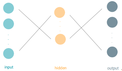
A Recurrent Neural Network is architected in the same way as a “traditional” Neural Network. We have some inputs, we have some hidden layers and we have some outputs.

The only difference is that each hidden unit is doing a slightly different function. So, let’s explore how this hidden unit works.

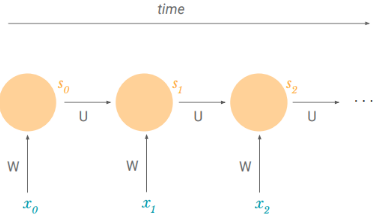
A recurrent hidden unit computes a function of an input and its own previous output, also known as the cell state. For textual data, an input could be a vector representing a word x(i) in a sentence of n words (also known as word embedding).

W and U are weight matrices and tanh is the hyperbolic tangent function.

Similarly, at the next step, it computes a function of the new input and its previous cell state: s2 = tanh(Wx1+ Us1). This behavior is similar to a hidden unit in a feed-forward Network. The difference, proper to sequences, is that we are adding an additional term to incorporate its own previous state.

A common way of viewing recurrent neural networks is by unfolding them across time. We can notice that we are using the same weight matrices W and U throughout the sequence. This solves our problem of parameter sharing. We don’t have new parameters for every point of the sequence. Thus, once we learn something, it can apply at any point in the sequence.

The fact of not having new parameters for every point of the sequence also helps us deal with variable-length sequences. In case of a sequence that has a length of 4, we could unroll this RNN to four timesteps. In other cases, we can unroll it to ten timesteps since the length of the sequence is not prespecified in the algorithm. By unrolling we simply mean that we write out the network for the complete sequence. For example, if the sequence we care about is a sentence of 5 words, the network would be unrolled into a 5-layer neural network, one layer for each word.

NB:

Sn, the cell state at time n, can contain information from all of the past timesteps: each cell state is a function of the previous self state which in turn is a function of the previous cell state. This solves our issue of long-term dependencies.
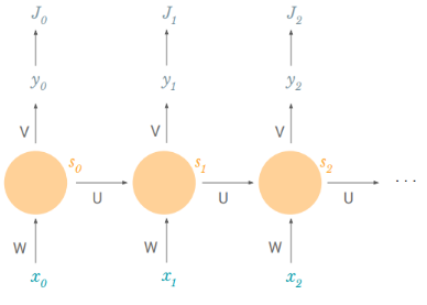
The above diagram has outputs at each time step, but depending on the task this may not be necessary. For example, when predicting the sentiment of a sentence, we may only care about the final output, not the sentiment after each word. Similarly, we may not need inputs at each time step. The main feature of an RNN is its hidden state, which captures some information about a sequence.

Now that we understand how a single hidden unit works, we need to figure out how to train an entire Recurrent Neural Network made up of many hidden units and even many layers of many hidden units.

How do we train a Recurrent Neural Network?

Let’s consider the following task: for a set of speeches in English, we need the model to automatically convert the spoken language into text i.e. at each timestep, the model produces a prediction of a transcript (an output) based on the part of speech at this timestep (the new input) and the previous transcript (the previous cell state).

Naturally, because we have an output at every timestep, we can have a loss at every timestep. This loss reflects how much the predicted transcripts are close to the “official” transcripts.

The total loss is just the sum of the losses at every timestep.

Since the loss is a function of the network weights, our task it to find the set of weights theta that achieve the lowest loss. For that, as explained in the first article “Introduction to Deep Learning”, we we can apply the gradient descent algorithm with backpropagation (chain rule) at every timestep, thus taking into account the additional time dimension.

W and U are our two weight matrices. Let us try it out for W.

Knowing that the total loss is the sum of the losses at every timestep, the total gradient is just the sum of the gradients at every timestep:

And now, we can focus on a single timestep to calculate the derivative of the loss with respect to W.

Easy to handle: we just use backpropagation.

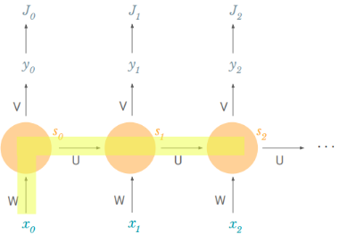
We remember that s2 = tanh(Wx1 + Us1) so s2 also depends on s1 and s1 also depends on W. This actually means that we can not just leave the derivative of s2 with respect to W as a constant. We have to expand it out farther.

So how does s2 depend on W?

It depends directly on W because it feeds right in (c.f. above formula of s2). We also know that s2 depends on s1 which depends on W. And we can also see that s2 depends on s0 which also depends on W.

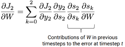
Thus, the derivative of the loss with respect to W could be written as follows:

We can see that the last two terms are basically summing the contributions of W in previous timesteps to the error at timestep t. This is key to understand how we model long-term dependencies. From one iteration to another, the gradient descent algorithm allows to shift network parameters such that they include contributions to the error from past timesteps.

For any timestep t, the derivative of the loss with respect to W could be written as follows:

So to train the model i.e. to estimate the weights of the network, we apply this same process of backpropagation through time for every weight (parameter) and then we use it in the process of gradient descent.

Why are Recurrent Neural Networks hard to train?

In practice RNNs are a bit difficult to train. To understand why, let’s take a closer look at the gradient we calculated above:

We can see that as the gap between timesteps gets bigger, the product of the gradients gets longer and longer. But, what are each of these terms?

Each term is basically a product of two terms: transposed W and a second one that depends on f’, the derivative of the activation function.

Initial weights W are usually sampled from standard normal distribution and then mostly < 1.
It turns out (I won’t prove it here but this paper goes into detail) that the second term is a Jacobian matrix because we are taking the derivative of a vector function with respect to a vector and its 2-norm, which you can think of it as an absolute value, has an upper bound of 1. This makes intuitive sense because our tanh (or sigmoid) activation function maps all values into a range between -1 and 1, and the derivative f’ is bounded by 1 (1/4 in the case of sigmoid).

Thus, with small values in the matrix and multiple matrix multiplications, the gradient values are shrinking exponentially fast, eventually vanishing completely after a few time steps. Gradient contributions from “far away” steps become zero, and the state at those steps doesn’t contribute to what you are learning: you end up not learning long-range dependencies.

Vanishing gradients aren’t exclusive to RNNs. They also happen in deep Feedforward Neural Networks. It’s just that RNNs tend to be very deep (as deep as the sentence length in our case), which makes the problem a lot more common.

Fortunately, there are a few ways to combat the vanishing gradient problem. Proper initialization of the Wmatrix can reduce the effect of vanishing gradients. So can regularization. A more preferred solution is to use ReLU instead of tanh or sigmoid activation functions. The ReLU derivative is a constant of either 0 or 1, so it isn’t as likely to suffer from vanishing gradients.

An even more popular solution is to use Long Short-Term Memory (LSTM) or Gated Recurrent Unit (GRU) architectures. LSTMs were first proposed in 1997 and are perhaps the most widely used models in NLP today. GRUs, first proposed in 2014, are simplified versions of LSTMs. Both of these RNN architectures were explicitly designed to deal with vanishing gradients and efficiently learn long-range dependencies. We’ll cover them in the next part of this article.

It will come soon!

Originally posted here.

Resources I used when writing this article:

DSC Resources

Sequence Modeling with Neural Networks – Part I