
Hello! I like to share my interesting experience While I was working as a junior Data Scientist, I can even say I was a beginner during that time in this data science domain.
One of the customers came to us for machine learning implementation for their problem statement in either way unsupervised and supervised forms, I thought it was going to be as usual mode of execution and process because based on my experience for small scale implementation or during my training period we use to have 25-30 features and we play around with that and we use to predict or classify or clustering the dataset and share the outcome.
But this time they come up with thousands of features, But I was a little surprised and scared about the implementation and my head started spinning as anything. Same time my Senior Data Scientist brought everyone from the team into the meeting room.
My Senior Data Scientist (Sr. DS) coined the new word to us, that is nothing but Dimensionality Reduction (OR) Dimension Reduction (OR) Curse Of Dimensionality, all beginners thought that he is going to explain something in Physis, we had little remembrance that we had come across this term during our training programme. then he started to sketch on the board (Refer fig-1). When we started looking at 1-D, 2-D we are much comfortable but 3-D and above our heads started to spin.
 1-D and 2-D
 3 D
3 DSr. DS has continued his lecture, all these sample pictures are just notable features and we could play around with these, in a real-time scenario, many Machine Learning(ML) problems involve thousands of features, so we end up training those models became extremely slow and will not give good solutions for business problem and we couldnt freeze the model, this situation is the so-called Curse Of Dimensionality working. Then we all started asking a question that how we should handle this.
He took a long breath and continue to share his experience in his own style. He started with a simple definition as follows.
What is Dimensionality?
We can say the number of features in our dataset is referred to as its dimensionality.
What is Dimensionality Reduction?
Dimensionality Reduction is the process of reducing the dimensions(features) of a given dataset. Lets say if your dataset with a hundred columns/features and bringing the number of columns down to 20-25. In simple terms, you are converting the Cylinder/Sphere to a Circle or Cube into a Plane in the two-dimensional space as below figure.
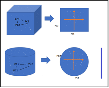 Converting 3D- 2D
He has drawn below the relationship clearly between Modle Performance and Number of Features(Dimensions). As the number of features increases, the number of data points also increases proportionally. the straight statement is that the more features will bring more data samples, So we have represented all combinations of features and their values.
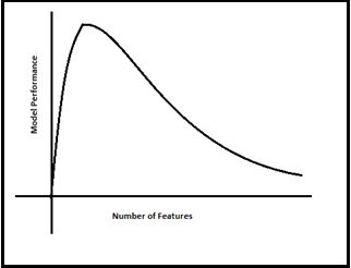 Modle Performance Vs Number of Features
Now everyone in the room got the feel of what is Curse Of Dimensionality at a very high level.
Benefits of doing Dimensionality Reduction
Suddenly, one of the team members asked can he tell us the benefits of doing dimensionality reduction in the given dataset.
Our Sr. DS didnt stop sharing his extensive knowledge further. He has continued as below.
There are lots of benefits if we go with dimensionality reduction.
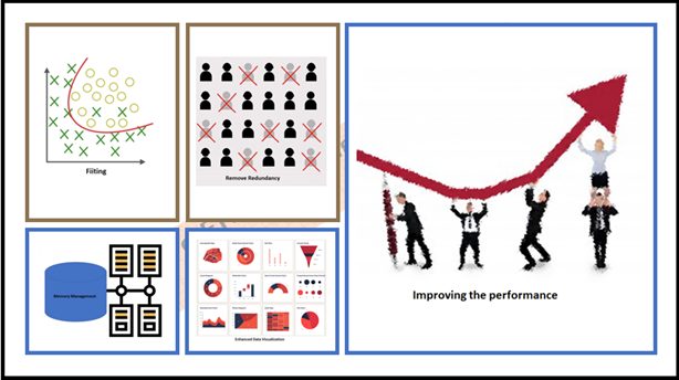
- It helps to remove redundancy in the features and noise error factors ultimately enhanced visualization of the given data set.
- Excellent memory management activity has been exhibited due to dimensionality reduction.
- Improving the performance of the model by choosing the right features by removing the unnecessary lists of features from the dataset.
- Certainly, less number of dimensions (mandatory list of dimensions) required less computing efficiency and train the model faster with improved model accuracy.
- Considerably reducing the Complexity and Overfitting of the overall model and its performance.
Yes! it was an awe-inspiring spectacle, robustness, and dynamics of the Dimensionality Reduction. Now I can visualization the overall benefit as below. hope it could help you too
Benefits of Dimensionality Reduction.
What is next, Of Course! We jump into the next major question that what are techniques available for Dimensionality Reduction.
Dimensionality Reduction Techniques
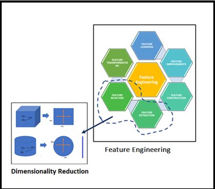
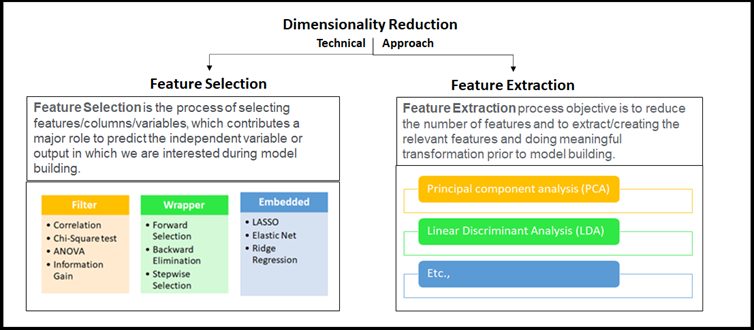
Our Sr. DS very much interested continued his explanation on the techniques whichever possible in Data Science domain, broadly classified into two approaches as mentioned earlier considering selecting the best-fit Feature(s) or removing less important Feature in the given high dimensional dataset. these high-level techniques use to be called Feature Selection or Feature Extraction, and basically, this is part of Feature Engineering. He has connected the dots perfectly.
 Locating Dimensionality Reduction in Feature Engineering family
He took us further in-depth concepts to understand the big picture of applied Dimensionality Reduction on the high dimensional dataset. Once we saw the below figure we able to relate the Feature Engineering and Dimensionality Reduction. Look at this figure the essence of Dimensionality Reduction well by our Sr. DS is in it!
Everyone was interested to know how to apply all these using Phyton libraries with the help of simple coding. our Sr. DS asked me to bring colorful markers and dusters

Sr. DS picked up the new blue marker and started explaining PCA with a simple example as follows, before that he explained what is PCA stuff for dimensionality reduction.
Principal Component Analysis(PCA): PCA is a technique for dimensionality reduction of a given dataset, by increasing interpretability with negligible information loss. Here the number of variables is decreasing, so it makes further analysis simpler. Which converts a set of correlated variables to a set of uncorrelated variables. Used for machine learning predictive modeling. And he advised us to go through Eigenvector, Eigen Values
He took familiar wines.csv for his quick analysis.

# Import all the necessary packages
import pandas as pd
 import numpy as np
 import matplotlib.pyplot as plt
 import seaborn as sns from sklearn.model_selection
 import train_test_split from sklearn.linear_model
 import LinearRegression from sklearn.metrics
 import confusion_matrix from sklearn.metrics
 import accuracy_score from sklearn
 import metrics %matplotlib inline
 import matplotlib.pyplot as plt
 %matplotlib inline

 wq_dataset = pd.read_csv('winequality.csv')
EDA on a given data set
wq_dataset.head(5)

wq_dataset.describe()

wq_dataset.isnull().any()
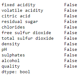
No Null value in the given data set, So great and were lucky.
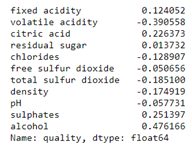
Find correlations of each feature
correlations = wq_dataset.corr()['quality'].drop('quality') print(correlations)
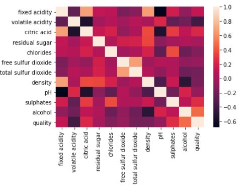
Correlation Representation using Heatmap
sns.heatmap(wq_dataset.corr()) plt.show()
x = wq_dataset[features] y = wq_dataset['quality']
[fixed acidity, volatile acidity, citric acid, chlorides, total sulfur dioxide, density, sulphates, alcohol]
x_train, x_test, y_train, y_test = train_test_split(x, y, random_state=3)
Training and Testing Shape
print('Traning data shape:', x_train.shape) print('Testing data shape:', x_test.shape)
Traning data shape: (1199, 8) Testing data shape: (400, 8)
PCA implementation for Dimensionality reduction (with 2 columns)
from sklearn.decomposition import PCA pca_wins = PCA(n_components=2) principalComponents_wins = pca_wins.fit_transform(x)
Naming them as principal component 1, principal component 2
pcs_wins_df = pd.DataFrame(data = principalComponents_wins, columns = ['principal component 1', 'principal component 2'])
New principal components and their values.
pcs_wins_df.head()
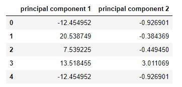
We all surprised when looking at the above two columns with new column name and values, We asked what happen to fixed acidity, volatile acidity, citric acid, chlorides, total sulfur dioxide, density, sulphates, alcohol columns. Sr. DS said all gone, now we have just two columns after we applied PCA for dimensionality reduction on given data and we are going to implement few models and this is going to be the normal way.
He has mentioned one keyword variation per principal component
this is the fraction of variance explained by a principal component is the ratio between the variance of that principal component and the total variance.
print('Explained variation per principal component: {}'.format(pca_wins.explained_variance_ratio_))
Explained variation per principal component: [0.99615166 0.00278501]
Followed by this he was demonstrated the following models
- Logistic Regression
- Random forest
- KNN
- Naive Bayes
Accuracy was better and little difference among each model, but he has mentioned this is for PCA implementation. Everyone in the room felt that we have completed an excellent roller coaster. he has advised us to do hands-on other Dimensionality Reduction Techniques.

Okay, Guys! Thanks for your time, hope I able to narrate my learning experience of Dimensionality Reduction Techniques in right ways here, I trust it would help to continue the journey to handle complex data set in machine learning problem statement. Cheers!
