Python and R are the two most commonly used languages for data science today. They are both fully open source products and completely free to use and modify as required under the GNU public license.
But which one is better? And, more importantly, which one should you learn?
Both are widely used and are standard tools in the hands of every data scientist.
The answer may surprise you – because as a professional data scientist, you should be ready to deal with both.
Python has certain use cases and so does R. The scenarios in which they are used vary. It is more often the environment and the needs of the client or your employer which dictates the choice between Python and R. Many things are easier in Python. But R also has its place in your development toolkit.
Python
Python is a general-purpose programming language released by Guido Van Rossum in 1991.
Since then, Python has been used in multiple environments for multiple purposes, including, but not limited to:
● Web Development (Django)
● Web Microservices (Flask)
● Zappa Serverless Framework for Python
● TensorFlow (Deep Learning Machine Learning Models)
● Keras (High-Level Abstractions to Simplify TensorFlow Development)
● Popular apps built in Python include Dropbox, BitTorrent, Morpheus, Calibre, Blender, and Mercurial – among many, many others.
Python has more appeal for software engineers. This is mainly because industry use, production-ready code can be usually written in Python. If you have the background of a software engineer or already know programming, Data Science in Python is a better choice for you (especially if you’re a beginner).
Another situation where Python shines is the sheer number pre-existing libraries that are readily available and open sourced to use. The large number of packages available in the PyPI (short for Python Package Index) repository with over 121k packages that automate many programming tasks at various levels of abstraction, making life easy for the programmer. At least 6k out of the packages on PyPI are focused on data science. Python also excels in readability. Compared to R, Python is much easier to read and to understand. Python is faster than R, in some cases dramatically faster.
R
R is a statisticians programming language designed for statisticians by statisticians. It originated in the ‘90s through George Ross Ihaka and Robert Gentleman. R excels in academic use and in the hands of a statistician. People who have formal training in Statistics, such as a Statistics degree, find working with R extremely simple. The repository for R packages or libraries, called CRAN (Comprehensive R Archive Network) contains nearly 12k packages, roughly half of which are for data science with R. R also excels at data visualization. Analyzing data on a one-time basis is often simpler and more easily expressible in R.
Also, once upon a time, using Python meant linking many libraries together, some of which would become incompatible after feature revisions and library updates. That is no longer true because of Anaconda – see below. For a short time, deep learning was strictly a Python feature – which shifted the balance of the machine learning world towards Python, for a short time. However, with the release of Keras for TensorFlow in R, that factor changed as well, and deep learning models could now be used in R.
So, what is the answer? Which one should you use?
The answer – both.
Jupyter Notebook – Integrating Python and R

The Anaconda distribution from Continuum Analytics has completely disrupted the machine learning picture. Anaconda supports the standard libraries required for Python and machine learning – NumPy, SciPy, Pandas, SymPy, Seaborn, Matplotlib – as well as full support for R with an outstanding IDE called R Studio.
For Deep Learning it supports TensorFlow, Theano, Caffe, Scikit-Learn, and Torch. One of its most remarkable features is the introduction of the Jupyter Notebook, an integrated platform which supported the use of Python and R in the same environment while keeping everything open source.
Another option is the Hydrogen plug-in for the Atom text editor. It allows you to enter any code that you can use in a Jupyter Notebook and returns the result in the editor. However, it is still in alpha and crashed with an error on my local machine. The Jupyter Lab application allows Python and R notebook editing in the same environment, using the concept of separate and even remote kernels.
As the machine learning field progresses, one can expect more plugins like Hydrogen (which I can’t wait to test once it’s out of alpha) produced in the very near future. So, Python excels in machine learning, while R excels in statistics.
But why should you learn both?
Because a professional data scientist needs to understand statistics and the mathematics behind the machine learning algorithms in great detail.
We shall examine two SVM machine learning models, one through Python code, and then another through R code. This will give us a good picture of how both languages work.
Python Code
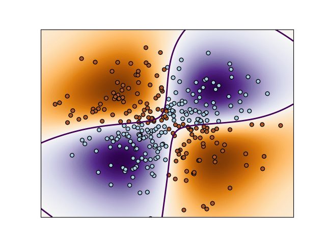
This code performs binary classification using non-linear support vector machine using a Gaussian kernel. The target to predict is a XOR of the inputs.
The color map illustrates the decision function learned by the Support Vector Machine Classifier. (SVC)
print(__doc__)
import numpy as np
import matplotlib.pyplot as plt
from sklearn import svm
xx, yy = np.meshgrid(np.linspace(-3, 3, 500),
np.linspace(-3, 3, 500))
np.random.seed(0)
X = np.random.randn(300, 2)
Y = np.logical_xor(X[:, 0] > 0, X[:, 1] > 0)
# fit the model
clf = svm.NuSVC()
clf.fit(X, Y)
# plot the decision function for each datapoint on the grid
Z = clf.decision_function(np.c_[xx.ravel(), yy.ravel()])
Z = Z.reshape(xx.shape)
plt.imshow(Z, interpolation=’nearest’,
extent=(xx.min(), xx.max(), yy.min(), yy.max()), aspect=’auto’,
origin=’lower’, cmap=plt.cm.PuOr_r)
contours = plt.contour(xx, yy, Z, levels=[0], linewidths=2,
linetypes=’–‘)
plt.scatter(X[:, 0], X[:, 1], s=30, c=Y, cmap=plt.cm.Paired,
edgecolors=’k’)
plt.xticks(())
plt.yticks(())
plt.axis([-3, 3, -3, 3])
plt.show()
.Output:

R Code
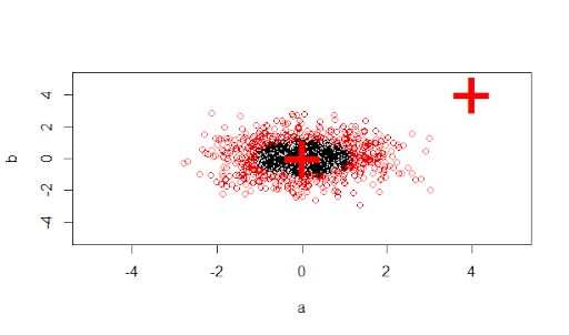
This program uses the iris dataset to illustrate the use of a non-linear SVM classifier. This code is deliberately a little more complex since it applies ML techniques to a full-fledged built in dataset – the iris dataset – one of the canonical data sets used to illustrate the capacities of the ML techniques traditionally. THis code also illustrates the usage of the built-in statistical functions of R.
You will need to install R package e1071 and add it to the compile list by calling library(e1071) before executing the code below. But don’t worry – installing new packages in R Studio is ridiculously simple.
# NOT RUN {
data(iris)
attach(iris)
## classification mode
# default with factor response:
library(e1071)
#loads the svm library into the compile path
model <- svm(Species ~ ., data = iris)
# alternatively the traditional interface:
x <- subset(iris, select = -Species)
y <- Species
model <- svm(x, y)
print(model)
summary(model)
# test with train data
pred <- predict(model, x)
# (same as:)
pred <- fitted(model)
# Check accuracy:
table(pred, y)
.Output:
y
pred setosa versicolor virginica
setosa 50 0 0
versicolor 0 48 2
virginica 0 2 48
<code>
# visualize (classes by color, SV by crosses):
plot(cmdscale(dist(iris[,-5])),
col = as.integer(iris[,5]),
pch = c(“o”,“+”)[1:150 %in% model$index + 1])
## try regression mode on two dimensions
# create data
x <- seq(0.1, 5, by = 0.05)
y <- log(x) + rnorm(x, sd = 0.2)
# estimate model and predict input values
m <- svm(x, y)
new <- predict(m, x)
# visualize
plot(x, y)
points(x, log(x), col =2)
points(x, new, col = 4)
## density-estimation
# create 2-dim. normal with rho=0:
X <- data.frame(a = rnorm(1000), b = rnorm(1000))
attach(X)
# traditional way:
m <- svm(X, gamma =0.1)
# formula interface:
m <- svm(~., data = X, gamma =0.1)
# or:
m <- svm(~ a + b, gamma =0.1)
# test:
newdata <- data.frame(a = c(0, 4), b = c(0, 4))
predict (m, newdata)
# visualize:
plot(X, col =1:1000 %in% m$index + 1, xlim = c(-5,5), ylim=c(-5,5))
points(newdata, pch =“+”, col = 2, cex = 5)
i2 <- iris
levels(i2$Species)[3] <-“versicolor”
summary(i2$Species)
wts <-100 / table(i2$Species)
wts
m <- svm(Species ~ ., data = i2, class.weights = wts)
# }
Output:

As you can see, the R code is fundamentally more powerful in its graphing and statistical abilities than Python. Being a language of statisticians by statisticians, if you have a statistics background, using R will be the best launchpad for your new career in data science.
Conclusion
Thus, when it comes to choosing between Python and R, any data scientist who is worth his money will know that he is supposed to know both.
And in the end, all the most advanced software engineering skills won’t get you anywhere unless you have a firm foundation in Statistics – or a professional statistician in your team. The main reason that we use analytics is to make business decisions. And we can utilize it best when we have an iron-clad grasp of the entire picture.
So, on Python versus R, to sum up:
Both perform similar tasks in data science but are optimized toward different domains. If you are a software engineer, choose Python. If you are an academic researcher, choose R.
And if you are a data scientist – choose both.
Original Article Published here
