Many Machine Learning articles and papers describe the wonders of the Support Vector Machine (SVM) algorithm. Nevertheless, when using it on real data trying to obtain a high accuracy classification, I stumbled upon several issues.
I will try to describe the steps I took to make the algorithm work in practice.
This model was implemented using R and the library “e1071”.
To install and use it type:
> install.packages(“e1071”)
> library(“e1071”)
When you want to classify data in two categories, few algorithms are better than SVM.
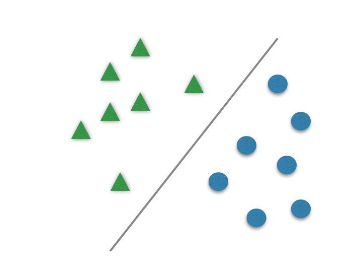
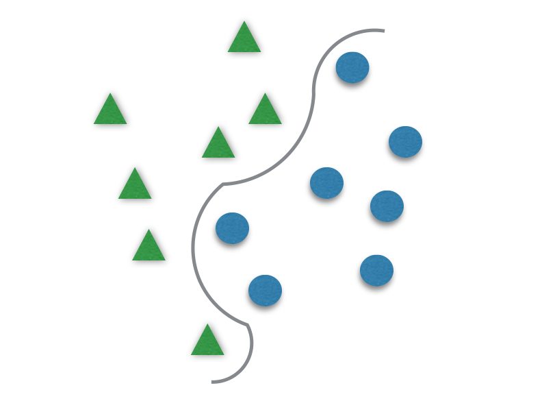
It usually divides data in two different sets by finding a “line” that better separates the points. It is capable to classify data linearly (put a straight line to differentiate sets) or do a nonlinear classification (separates sets with a curve). This “separator” is called a hyperplane.
Normalize Features
Before you even start running the algorithm, the first thing needed is to normalize your data features. SVM uses features to classify data, and these should be obtained by analyzing the dataset and seeing what better represents it (like what is done with SIFT and SURF for images). You might want to use/combine the mean value, the derivative, standard deviation or several other ones. When parameters are not normalized, the ones with greater absolute value have greater effect on the hyperplane margin. This means that some parameters are going to influence more your algorithms than others. If that is not what you want, make sure all data features have the same value range.
Another important point is to check the SVM algorithm parameters. As many Machine Learning algorithms, SVM has some parameters that have to be tuned to gain better performance. This is very important: SVM is very sensitive to the choice of parameters. Even close parameters values might lead to very different classification results. Really! In order to find the best for your problem, you might want to test some different values. A great tool to help this job in R is the tune.svm() method. It can test several different values, and return the ones which minimizes the classification error for the 10-fold cross validation.
Example of tune.svm() output:
The γ (gama) has to be tuned to better fit the hyperplane to the data. It is responsible for the linearity degree of the hyperplane, and for that, it is not present when using linear kernels. The smaller γ is, the more the hyperplane is going to look like a straight line.If γ is too great, the hyperplane will be more curvy and might delineate the data too well and lead to overfitting.
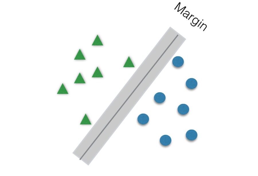
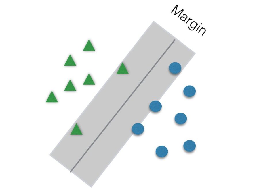
Another parameter to be tuned to help improve accuracy is C. It is responsible for the size of the “soft margin” of SVM. The soft margin is a “gray” area around the hyperplane. This means that points inside this soft margin are not classified as any of the two categories. The smaller the value of C, the greater the soft margin.
How to Prepare Data
The svm() method in R expects a matrix or dataframe with one column identifying the class of that row and several features that describes that data. The following table shows an example of two classes, 0 and 1, and some features. Each row is a data entry.
class f1 f2 f3
1 0 0.100 0.500 0.900
2 0 0.101 0.490 0.901
3 0 0.110 0.540 0.890
4 0 0.100 0.501 0.809
5 1 0.780 0.730 0.090
6 1 0.820 0.790 0.100
7 1 0.870 0.750 0.099
8 1 0.890 0.720 0.089
The input for the svm() method could be:
> svm(class ~., data = my_data, kernel = “radial”, gamma = 0.1, cost = 1)
Here “class” is the name of the column that describes the classes of your data and “my_data” is obviously your dataset. The parameters should be the ones best suitable for your problem.
Test Your Results
Always separate a part of your data to test. It is a common practice to get 2/3 of data as training set (to find your model) and 1/3 as test set. Your final error should be reported based on the test set, otherwise it can be biased.
You can divide your data in R like the following example:
> data_index <- 1:nrow(dataset)
> testindex <- sample(data_index, trunc(length(data_index)*30/100))
> test_set <- dataset[testindex,]
> train_set <- dataset[-testindex,]
> my_model <- svm(class ~., data = train_set, kernel = “radial”, gamma = 0.1, cost = 1)
And then to test the results on the test_set:
> my_prediction <- predict(my_model, test_set[,-1])
test_set[,-1] removes the first column (the class column) to make the predictions only based on the features of the data. You should remove the column that labels your data.
Final Considerations
- The tune.svm() method might take a while to run depending on your data size. Nevertheless, usually it is worth it.
- We usually use logarithmically spaced values for the SVM parameters, varying from 10^-6 to 10^6. Here are some explanations: http://stats.stackexchange.com/questions/81537/gridsearch-for-svm-p…
- If you try to run tune.svm() with a dataset of less than 10 rows, you will get this error:
Error in tune(“svm”, train.x = x, data = data, ranges = ranges, …) :
‘cross’ must not exceed sampling size!
So make sure you add more lines to this data test.
More about SVM
https://en.wikibooks.org/wiki/Data_Mining_Algorithms_In_R/Classific…
http://rischanlab.github.io/SVM.html
https://cran.r-project.org/web/packages/e1071/vignettes/svmdoc.pdf
http://pyml.sourceforge.net/doc/howto.pdf
http://neerajkumar.org/writings/svm/
Post from:
http://girlincomputerscience.blogspot.com/2015/02/svm-in-practice.html


