This article was written by Jason Brownlee.
Artificial neural networks are a fascinating area of study, although they can be intimidating when just getting started. There are a lot of specialized terminology used when describing the data structures and algorithms used in the field. In this post you will get a crash course in the terminology and processes used in the field of multi-layer perceptron artificial neural networks. After reading this post you will know:
- The building blocks of neural networks including neurons, weights and activation functions.
- How the building blocks are used in layers to create networks.
- How networks are trained from example data.
Let’s get started.
Source for picture: click here
Crash Course Overview:
We are going to cover a lot of ground very quickly in this post. Here is an idea of what is ahead:
- Multi-Layer Perceptrons.
- Neurons, Weights and Activations.
- Networks of Neurons.
- Training Networks.
We will start off with an overview of multi-layer perceptrons.
1. Multi-Layer Perceptrons
The field of artificial neural networks is often just called neural networks or multi-layer perceptrons after perhaps the most useful type of neural network. A perceptron is a single neuron model that was a precursor to larger neural networks.
It is a field that investigates how simple models of biological brains can be used to solve difficult computational tasks like the predictive modeling tasks we see in machine learning. The goal is not to create realistic models of the brain, but instead to develop robust algorithms and data structures that we can use to model difficult problems.
The power of neural networks come from their ability to learn the representation in your training data and how to best relate it to the output variable that you want to predict. In this sense neural networks learn a mapping. Mathematically, they are capable of learning any mapping function and have been proven to be a universal approximation algorithm.
The predictive capability of neural networks comes from the hierarchical or multi-layered structure of the networks. The data structure can pick out (learn to represent) features at different scales or resolutions and combine them into higher-order features. For example from lines, to collections of lines to shapes.
2. Neurons
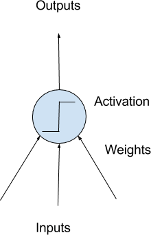
The building block for neural networks are artificial neurons. These are simple computational units that have weighted input signals and produce an output signal using an activation function.

Model of a Simple Neuron
Neuron Weights:
You may be familiar with linear regression, in which case the weights on the inputs are very much like the coefficients used in a regression equation.
Like linear regression, each neuron also has a bias which can be thought of as an input that always has the value 1.0 and it too must be weighted.
For example, a neuron may have two inputs in which case it requires three weights. One for each input and one for the bias.
Weights are often initialized to small random values, such as values in the range 0 to 0.3, although more complex initialization schemes can be used.
Like linear regression, larger weights indicate increased complexity and fragility. It is desirable to keep weights in the network small and regularization techniques can be used.
Activation:
The weighted inputs are summed and passed through an activation function, sometimes called a transfer function.
An activation function is a simple mapping of summed weighted input to the output of the neuron. It is called an activation function because it governs the threshold at which the neuron is activated and strength of the output signal.
Historically simple step activation functions were used where if the summed input was above a threshold, for example 0.5, then the neuron would output a value of 1.0, otherwise it would output a 0.0.
Traditionally non-linear activation functions are used. This allows the network to combine the inputs in more complex ways and in turn provide a richer capability in the functions they can model. Non-linear functions like the logistic also called the sigmoid function were used that output a value between 0 and 1 with an s-shaped distribution, and the hyperbolic tangent function also called tanh that outputs the same distribution over the range -1 to +1.
More recently the rectifier activation function has been shown to provide better results.
3. Networks of Neurons
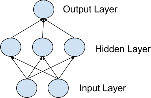
Neurons are arranged into networks of neurons. A row of neurons is called a layer and one network can have multiple layers. The architecture of the neurons in the network is often called the network topology.

Model of a Simple Network
Input or Visible Layers:
The bottom layer that takes input from your dataset is called the visible layer, because it is the exposed part of the network. Often a neural network is drawn with a visible layer with one neuron per input value or column in your dataset. These are not neurons as described above, but simply pass the input value though to the next layer.
Hidden Layers:
Layers after the input layer are called hidden layers because that are not directly exposed to the input. The simplest network structure is to have a single neuron in the hidden layer that directly outputs the value.
Given increases in computing power and efficient libraries, very deep neural networks can be constructed. Deep learning can refer to having many hidden layers in your neural network. They are deep because they would have been unimaginably slow to train historically, but may take seconds or minutes to train using modern techniques and hardware.
Output Layer:
The final hidden layer is called the output layer and it is responsible for outputting a value or vector of values that correspond to the format required for the problem.
The choice of activation function in he output layer is strongly constrained by the type of problem that you are modeling. For example:
- A regression problem may have a single output neuron and the neuron may have no activation function.
- A binary classification problem may have a single output neuron and use a sigmoid activation function to output a value between 0 and 1 to represent the probability of predicting a value for the class 1. This can be turned into a crisp class value by using a threshold of 0.5 and snap values less than the threshold to 0 otherwise to 1.
- A multi-class classification problem may have multiple neurons in the output layer, one for each class (e.g. three neurons for the three classes in the famous iris flowers classification problem). In this case a softmax activation function may be used to output a probability of the network predicting each of the class values. Selecting the output with the highest probability can be used to produce a crisp class classification value.
4. Training Networks
Once configured, the neural network needs to be trained on your dataset.
To read the full original article (and learn more about data preparation, stochastic gradient descent, and weight updates) click here. For more neural network related articles on DSC click here.
DSC Resources
- Services: Hire a Data Scientist | Search DSC | Classifieds | Find a Job
- Contributors: Post a Blog | Ask a Question
- Follow us: @DataScienceCtrl | @AnalyticBridge
Popular Articles

