Beautiful Mathematical Images

To zoom in on any picture, click on the image to get a higher resolution.

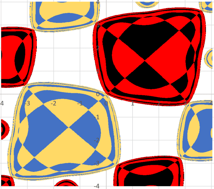
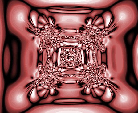
Figure 1: The pillow basins (see section 3)

The topic discussed here is closely related to optimization techniques in machine learning. I will also talk about dynamic systems, especially discrete chaotic ones, in two dimensions. This is a fascinating branch of quantitative science, with numerous applications. This article provides you with an opportunity to gain exposure to this discipline, which is usually overlooked by data scientists but well studied by mathematicians and physicists. The images presented here are selected not just for their beauty, but most importantly for their intrinsic value: the practical insights that can be derived from them, and the implications for machine learning professionals. 

1. Introduction to dynamical systems

A discrete dynamical system is a sequence xn+1 = f(xn) where n is an integer, starting with n = 0 (the initial condition) and where f is a real-valued function. In the continuous version (not discussed here), the index n (also called time) is a real number. The function f is called the map of the system, the system itself is also called a mapping: the most studied one is the logistic map defined by f(x) = ρx (1 – x), with x in [0, 1]. When ρ = 4, it is fully chaotic. The sequence (xn) for a specific initial condition x0, is called the orbit. 

Another example of chaotic mapping is the digits in base b of an irrational number z in [0,1]. In this case, x0 = z, f(x) = bx – INT(bx) and the n-th digit of z is INT(bxn). Here INT is the integer part function. It is studied in details in my book Applied Stochastic Processes, Chaos Modeling, and Probabilistic Properties of Numeration Systems, available for free, here. See also the second, large appendix in my free book Statistics: New Foundations, Toolbox, and Machine Learning Recipes, available here. Applications include the design of non-periodic pseudo-random number generators, cryptography, and even a new concept of number guessing (gambling or simulated stock market) where the winning numbers can be computed in advance with a public algorithm that requires trillions of years of computing time, while a fast, private algorithm is kept secret. See here. 

The concept easily generalizes to two dimensions. In this case xn is a vector or a complex number. Mappings in the complex plane are known to produce beautiful fractals; it has been used in fractal compression algorithms, to compress images. In one dimension, once in chaotic mode, they produce Brownian-like orbits, with applications in Fintech.

1.1. The sine map

Moving forward, we focus exclusively on a particular case of the sine mapping, both in one and two dimensions. This is one of the most simple nonlinear mappings, yet it is very versatile and produces a large number of varied and intriguing configurations. In one dimension, it is defined as follows:

xn+1 = –ρxn + λ sin(xn).

In two dimensions, it is defined as

xn+1 = –ρxn + λ sin(yn),

yn+1 = –ρxn + λ sin(xn).

This system is governed by two real parameters: ρ and λ. Some of its properties and references are discussed here. 

2. Connection to machine learning optimization algorithms

I need to introduce two more concepts before getting down to the interesting stuff. The first one is called fixed point. Note that a root is simply a value x* such that f(x*) = 0. Some systems don’t have any root, some have one, some have several, and some have infinitely many, depending on the values of the parameters (in our case, depending on ρ and λ, see section 1.1). Some or all roots can be found using the following fixed point recursion: xn+1 = xn + f(xn). In our case, this translates to using the following algorithm.

2.1. Fixed point algorithm

For our sine mapping defined in section 1.1, proceed as follows

xn+1 = xn – ρxn + λ sin(xn)

in one dimension, or 

xn+1 = xn – ρxn + λ sin(yn),

yn+1 = xn – ρxn + λ sin(xn),

in two dimensions. If the sequences in question converge to some x* (one dimension) or x*, y* (two dimensions), then the limit in question is a fixed point of the system. To find as many fixed points as possible, you need to try many different initial conditions. Some initial conditions lead to one fixed point, some lead to another fixed point, some lead to nowhere. Some fixed points can never be reached no matter what initial conditions you use. This is illustrated later in this article. 

2.2. Connection to optimization algorithms

Optimization techniques are widely used  in machine learning and statistical science, for instance in deep neural networks, or if you want to find a maximum likelihood estimator.

When looking for the maxima or minima of a function f, you try to find the roots of the derivative of f (in one dimension) or by vanishing its gradient (in two dimensions). This is typically done using the Newton Raphson method, which is a particular type of fixed point algorithm, with quadratic convergence.

2.3. Basins of attraction

The second concept I introduce is basins of attraction. A basin of attraction is the full set of initial conditions such that when applying the fixed point algorithm in section 2.2, the fixed point iterations always converge to the same root x* of the system.

Let me illustrate this with the one-dimensional sine mapping, with ρ = 0 and λ = 1. The roots of the system are solutions to sin(x) = 0, that is x* = kπ, where k is any positive or negative integer. If the initial condition x0 is anywhere in the open interval ]2kπ, 2(k+1)π[, then the fixed point algorithm always converge to the same x* = (2k + 1)π. So each of these intervals constitute a distinct basin of attraction, and there are infinitely many of them. However, none of the roots x* = 2kπ can be reached regardless of the initial condition x0, unless x0 = x* = 2kπ itself. 

In two dimensions, the basins of attractions look beautiful when plotted. Some have fractal boundaries. I believe none of their boundaries have an explicit, closed-form equation, except in trivial cases. This is illustrated in section 3, featuring the beautiful images promised at the beginning. 

2.4. Final note about the one-dimensional sine map

The sequence xn+1 = xn + λ sin(xn) behaves as follows. Here we assume λ   >  0 and ρ = 0.

• If λ  <  1, it converges to a root x*
• If λ  =  4, it oscillates constantly in a narrow horizontal band, never converging
• If λ  >  6, it behaves chaotically as a Brownian motion, unbounded, with the following exception below

There is a very narrow interval around λ  =  8, where behavior is non-chaotic. In that case, xn is asymptotically equivalent to +2π n or – 2π n, and the sign depends on the initial condition x0, and is very sensitive to it. In addition, for instance if x0 = 2 and λ = 8, then x2n – x2n-1 gets closer and closer to  α = 7.939712…, and x2n-1 – x2n-2 gets closer and closer to β = -1.65653… as n increases, with α + β = 2π. Furthermore, α satisfies the equation

For details, see here. The phenomenon in question is pictured in Figure 2 below. 

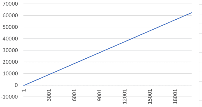
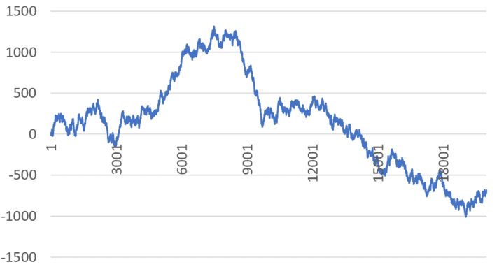
Figure 2: xn for n = 0 to 20,000 (X-axis), with x0 = 2; λ = 8 (top), λ = 7.98 (bottom)

3. Beautiful math images and their implications

The first picture (Figure 1, at the top of the article) features part of the four non-degenerate basins of attraction in the 2-dimensional sine map, when λ  =  2 and  ρ = 0.75. This sine map has 49 = 7 x 7 roots (x*, y*) with x* one of the 7 solutions of ρx = λ sin(λ sin(x) / ρ), and y* also one of the 7 solutions of the same equation. Computations were performed using the fixed point algorithm described in section 2.1. Note that the white zone corresponds to initial conditions (x0, y0) that do not lead to convergence of the fixed point algorithm. Each basin is assigned one color (other than white), and is made of sections of pillows with same color, scattered all over across many pillows. I call it the pillow basins. It would be interesting to see if the basin boundaries can be represented by simple mathematical functions. One degenerate basin (the fifth basin) consisting of the diagonal line x = y, is not displayed in Figure 1.

The picture below (Figure 3) shows parts of 5 of the infinitely many basins of attractions corresponding to λ = 0.5 and ρ  = 0, for the 2-dimensional site map. As in figure 1, the X-axis represents x0, the Y-axis represents y0. The range is from -4 to 4 both in Figure 1 and Figure 3. Each basin has its own color.

Figure 3: The octopus basins

In this case, we have infinitely many roots (with x*, y* being a multiple of  π) but only one-fourth of them can be reached by the fixed point algorithm. The more roots, the more basins, and as a result, the more interference between basins, making the image look noisy: a very small change in the initial conditions can lead to convergence to a different root, thus the overlapping between the basins. 

The take out from this is that when dealing with an optimization problem with many local maxima and minima, the solution you get is very sensitive to the initial conditions. In some cases, it matters, and in some cases it does not. If you are looking for a local optimum only, this is not an issue. This is further illustrated in Figure 4 below. It shows the orbits – that is the locations of (xn, yn) – starting with four different initial conditions (x0, y0), for the sine map featured in Figure 1. The blue dots represent a root (x*, y*). Each orbit except the green one converges to a different root. The green one oscillates back and forth, never converging.

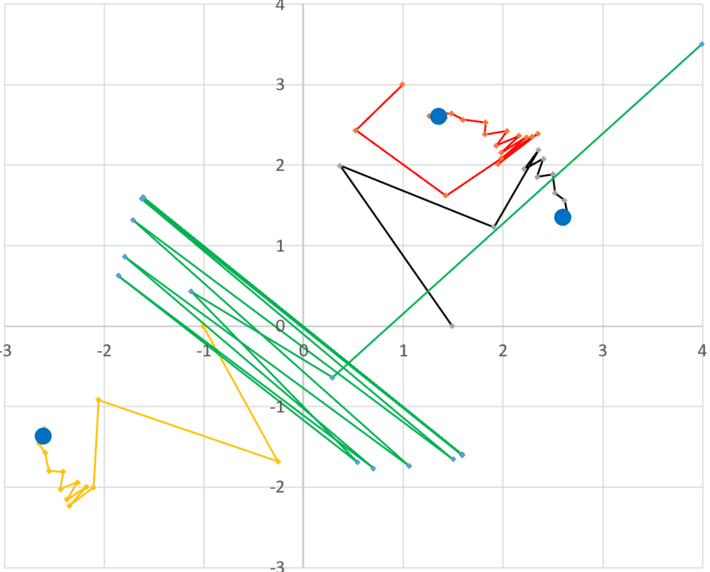
Figure 4: Four orbits corresponding to four initial conditions, for the case shown in Figure 1 

Note: When the system is very sensitive to initial conditions and highly chaotic, orbits computed numerically may be all wrong as round-off errors propagate exponentially fast as n increases. In that case, it is needed to use high precision computing to get accurate orbits, see here.

3.1. Benchmarking clustering algorithms

The basins of attractions can be used to benchmark supervised clustering algorithms. For instance, in Figure 1, if you group the red and black basins together, and the yellow and blue basins together, you end up with two well separated groups whose boundaries can be determined to arbitrary precision. One can sample points from the merged basins to create a training set with two groups, and check how well your clustering algorithm (based for instance on nearest neighbors or density estimation) can estimate the true boundaries. Another machine learning problem that you can test on these basins is boundary estimation: the problem consists in finding the boundary of a domain when you know points that are inside and points that are outside the domain. 

3.2. Interesting probability problem

The case pictured in Figure 1 leads to an interesting question. If you pick up randomly a vector of initial conditions (x0, y0), what is the probability that it will fall in (say) the red basin? It turns out that the probabilities are identical regardless of the basin. However, the probability to fall outside any basin (the white area) is different.

More beautiful images can be found in Part 2 of this article, here. To not miss them, subscribe to our newsletter, here. See also this article, featuring an image entitled “the eye of the Riemann Zeta function”. See also the Wikipedia article about “Infinite Compositions of Analytic Functions”, here. The picture below is from that article.

About the author:  Vincent Granville is a data science pioneer, mathematician, book author (Wiley), patent owner, former post-doc at Cambridge University, former VC-funded executive, with 20+ years of corporate experience including CNET, NBC, Visa, Wells Fargo, Microsoft, eBay. Vincent also founded and co-founded a few start-ups, including one with a successful exit (Data Science Central acquired by Tech Target). He is also the founder and investor in Paris Restaurant in Anacortes, WA. You can access Vincent’s articles and books, here.