In this article, I present a few modern techniques that have been used in various business contexts, comparing performance with traditional methods. The advanced techniques in question are math-free, innovative, efficiently process large amounts of unstructured data, and are robust and scalable. Implementations in Python, R, Julia and Perl are provided, but here we focus on an Excel version that does not even require any Excel macros, coding, plug-ins, or anything other than the most basic version of Excel. It is actually easily implemented in standard, basic SQL too, and we invite readers to work on an SQL version.
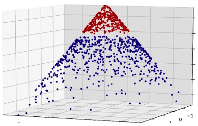
Source for picture: Logistic Regression vs Decision Trees vs SVM
1. Excel template for general machine learning
In short, we offer here an Excel template for machine learning and statistical computing, and it is quite powerful for an Excel spreadsheet. The techniques have been used by the author in automated data science frameworks (AI to automate content production, selection and scheduling for digital publishers) but also in the following contexts:
- spam detection,
- click, website, and keyword scoring (assigning a commercial value to a keyword, group of keywords, or content category)
- credit card fraud detection,
- Botnet detection, and predicting blog popularity.
The technique blends multiple algorithms that at first glance look traditional and math-heavy, such as decision trees, regression (logistic or linear) and confidence intervals. But they are radically different, can fit in a small spreadsheet (though the Python version is more powerful, flexible, and efficient), and do not involve math beyond high-school level. In particular, no matrix algebra is required to understand the methodology.
The methodology presented here is the result of 20 years worth of applied research on various large industrial data sets, where the author tried for years (eventually with success) to build a system that is simple and work. Most everyone else believed or made people believe that only complex system work, and have spent their time complexifying algorithms rather than simplifying them (partly for job security purposes.)
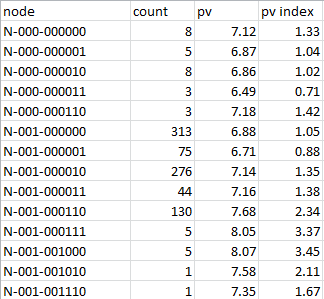
Node table (extract, from spreadsheet)
Who should use the spreadsheet?
First, the spreadsheet (as well as the Python, R, Perl or Julia version) are free to use and modify, even for commercial, purposes, or to make a product out of it and sell it. It is part of my concept of open patent, in which I share all my intellectual property publicly and for free.
The spreadsheet is designed as a tutorial, though it processes the same data set as the one used for the Python version. It is aimed at people that are not professional coders, people who manage data scientists, BI experts, MBA professionals, and people from other fields, with an interest in understanding the mechanics of some state-of-the-art machine learning techniques, without having to spend months or years learning mathematics, programming, and computer science. A few hours is needed to understand the details. This spreadsheet can be the first step to help you transition to a new, more analytical career path, or to better understand the data scientists that you manage or interact with. Or to spark a career in data science. Or even to teach machine learning concepts to high school students.
The spreadsheet also features a traditional technique (linear regression) for comparison purposes.
2. Description of the techniques used
Here we explain the differences between the standard and the Excel versions, and we provide an overview, at a high level, of the techniques being used, as well as why they are better in pretty much all applications, especially with unstructured and large data sets. Detailed descriptions are available in the articles referenced in this section.
Spreadsheet versus Python version
The Python version (also available in R, Perl and Julia) of the core technique is described here. Python / Perl offer the following advantages over Excel:
- It easily handles version 2.0 of HDT including overlapping nodes
- It easily handles big datasets, even in a distributed environment if needed
- It easily handles a large number of nodes
- Of course, it is incredibly faster for large data sets
The Excel version has the advantage of being interactive, and you can share it with people who are not data scientists.
But Excel (at least the template provided here) is mostly limited to nodes that form a partition of the feature space, that is, it is limited to non-overlapping nodes: see HDT version 1.0. So even if we have two nodes, one for the keyword data, and one for the keyword data science, in version 1,0, they are not overlapping: text buckets contain either data and not data science, or data science. In version 2.0, we no longer have this restriction. Note that nodes can be a combination of any number of keyword values or any other variables (called features in machine learning), and these variables can be quantitative or not.
For those familiar with computer science, nodes, both in the Excel or the Python version, are represented here as key-value pairs, typically stored as hash tables in Perl or Python, and as concatenated strings in Excel. For statisticians, nodes are just nodes of decision trees, though no tree structure is used (nor built) in my methodology — and this is why it is sometimes referred to as hidden decision trees (HDT). But you don’t need to understand this to use the methodology or understand how the spreadsheet works.
What is it about? What kind of algorithms are offered?
The methodology features an hybrid algorithm with essentially two components:
- Data aggregation into bins, based on sound feature selection, binning continuous and even discrete features, and metric design, not unlike decision trees. However, no tree is actually built, and the nodes may belong to several overlapping small decision trees, each one corresponding to a case or cluster easy to interpret. This is particularly true in HDT 2.0. I will call this the pseudo decision tree algorithm.
- Some kind of regression algorithm called Jackknife regression (see also here), but with much fewer parameters than in classical regression models, and more meaningful parameters, to avoid over-fitting and to be able to cope with cross-correlated features, while at the same time offering a simple interpretation. In the application discussed in the spreadsheet, one could argue that the Jackknife regression used is closer to logistic than linear regression as data is transformed using a log mapping, and we are trying to predict, for an article, the odds of being popular.
Data points belonging to a small node (say n < 10 observations) have the estimated / predicted response computed using the Jackknife regression (algorithm #2 above), the remaining points get scored using the pseudo-decision tree algorithm (algorithm #1 above.)
A lot of intelligence and creativity is put into creating great predictors (the features) and then perform sound feature selection. However, the features used in the spreadsheet and in the previous article on HDT (dealing with the same data set) will apply to all NLP (natural language processing) systems in numerous contexts.
In addition, while not incorporated in the spreadsheet, confidence intervals can be computed for each node with at least n observations (say n = 10) using percentiles for the response, computed for all data points (in this case, representing articles) in the node in question, see example at the bottom of section 3. This percentile function is even available in Excel. Then, data points in a node with too large a confidence interval are scored using the Jackknife regression rather than the pseudo decision tree. By scoring, I mean having the response estimated or predicted. By response, I mean the variable that we are trying to predict: in this case the page views number attached to an article (indeed, its logarithm, to smooth out big spikes due to external factors, or the fact that older articles have by definition more page views — see page view decay prediction for details.)
So no statistical theory is used anywhere in the methodology, not even to compute confidence intervals.
Why a brand new set of machine learning tools?
The HDT methodology offers the following advantages:
- The loss of accuracy, compared with standard procedures, is so small in the control data set, that it is negligible and much smaller than the inherent noise present in the data. This has been illustrated before on a different data set, and is confirmed again here (see next section.).
- The accuracy is much higher in the test data set, in a cross-validation framework where HDT is performed on a control data set, and performance measured on a different data set called test data set. So the methodology simply works better in the real world. This will be illustrated in an upcoming article, though the reason is easy to understand: HDT was designed as a robust method, to avoid over-fitting and issues caused by outliers, as well as to withstand model failures, messy data, and violations of assumptions.
In addition HDT also offers the following benefits:
- Easy interpretation of the results
- Simplicity, scalability, easy to implement in a distributed environment, and tested on unstructured big data
- No need to know statistical or mathematical theory to understand its inner workings
- Great to use as a machine learning tutorial for peple who do not code or not interesting in learning more about machine learning and coming from a different field (software engineering, management consulting, bioinformatics, econometrics, journalism, and so on.)
- Could be used in STEM programs in high schools, to give kids the chance to work on real machine learning problems using modern techniques.
- Few parameters to deal with, this is essentially a non-parametric, data-driven (as opposed to model-driven) technique.
- Since most companies use standard tools and software, using HDT can give you a competitive advantage (if you are allowed to choose your own method), and the learning curve is minimum.
Another way to highlight the benefits is to compare with Naive Bayes. Naive Bayes assumes that the features are independent. It is the workhorse of spam detection, and we all know how bad it performs. For instance, a message containing the keyword “breast cancer” is flagged because it contains the keyword “breast”, and Naive Bayes erroneously assumes that “breast” and “cancer” are independent. Not true with HDT.
Classical decision trees, especially the large ones with millions of nodes from just one single decision tree and involving more than 5 or 6 features at each final node, suffer from similar issues: over-fitting, artificial feature selection resulting in difficulties interpreting the results. maintenance challenges, over-parameterization making it more difficult to fine-tune, and most importantly, lack of robustness.
3. The Spreadsheet
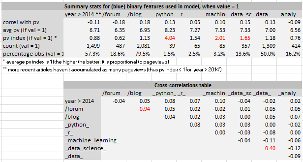
The data set and features used in this analysis are described here. The spreadsheet only uses a subset of the original features, as it is provided mostly as a template and for tutorial purposes. Yet even with this restricted set of features, it reveals interesting insights about some keywords (Python, R, data, data science) associated with popularity (Python being more popular than R), and some keywords that surprisingly, are not (keywords containing ”analy”, such as analytic.) Besides keywords found in the title, other features are used such as time of publication, and have also been binarized to increase stability and avoid an explosion in the number of nodes. Note that HDT 2.0 can easily handle a large number of nodes, and even HDT 1.0 (used in the spreadsheet) easily handles non-binary features.
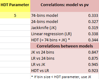
There are 2,616 observations (articles) and 74 nodes. By grouping all nodes with less than 10 observations into one node, we get down to 24 nodes. Interestingly, these small nodes perform much better than the average node. The correlations between the features and the response are very low, mostly because the keyword-like features trigger very few observations: very few articles contain the keyword R in the title (less than 3%.) As a result, the correlation between the response and predicted response is not high, around 0.33 regardless of the model. The solution is of course to add many more keywords to cover a much larger proportion of articles.
Notes
- In the Python version, keyword detection / selection (to create features) is part of the process, and included in the source code. Here, the keywords used as features are assumed to be pre-selected.
- Page view index (see spreadsheet) is a much better performance indicator than R-squared or correlation with response, to measure the predictive power of a feature. This is clearly the case with the feature “Python”.
- The Excel version is slightly different from the Python version, from a methodological point of view, as described in section 2.
- The goodness-of-fit for Jackknife and linear regression are very close, despite the fact that Jackknife is a very rough (but robust) approximation of linear regression.
- Jackknife has been used in its most elementary version, with only one M. When the cross-correlation structure is more complex, I recommend using Jackknife with two M’s as described here.
- Some of the features are correlated, for instance “being a blog” with “being a forum question”, or “containing data but not data science” with “containing data science”.
- When combining Jackknife with the pseudo-decision trees (applying Jackknife to small nodes) we get a result that is better than Jackknife, pseudo-decision trees, or linear regression taken separately.
- For much larger data sets that include all sorts (categories) of articles (not just about data science), I recommend creating and adding a feature called category. Such a feature can be build using an indexation algorithm.
- The response is denoted as pv.
Click here to get the spreadsheet. Below are some screenshots from the spreadsheet. Here pv is the response (logarithm of pageviews.)
Side Note: Confidence intervals for response (example)
Node N-100-000000 in the spreadsheet has an average pv of 5.85 (pv is the response), and consists of the following pv values: 5.10, 6.80, 5.56, 5.66, 6.19, 6.01, 5.56, 5.10, 6.80, 5.69. The 10th and 90th percentiles for pv are respectively 5.10 and 6.80, so [5.10, 6.80] is our confidence interval (CI) for this node. This computation of CI is similar to the methodology discussed here. This particular CI is well below the average pv — even the upper bound 6.80 is below the average pv of 6.83. In fact this node corresponds to articles posted after 2014, not a blog or forum question (it could be a video or event announcement), and with a title containing none of the keywords from the keyword feature list. The business question is: Should we continue to accept and promote such poor performing content? The answer is yes, but not as much as we used to. Competition is also dropping this kind of content for the same reasons, so, ironically, this is an opportunity to build a monopoly. Also variety is critical, and only promoting blogs that work well today is a recipe for long term failure, though it works well in the short term.
About the Author
Vincent Granville is a machine learning scientist, author and publisher. He was the co-founder of Data Science Central (acquired by TechTarget) and most recently, founder of Machine Learning Recipes.


