 In our last post, we explained the basics of streaming with Spark. Today, we want to talk about graphs and explore Apache Spark GraphX tool for graph computation and analysis. It is necessary to say that GraphX works only with Scala.
A graph is a structure which consists of vertices and edges between them. Graph theory finds its application in various fields such as computer science, linguistics, physics, chemistry, social sciences, biology, mathematics, and others. Problems connected with graph analysis are rather complicated, but there are many modern convenient instruments and libraries for these purposes.
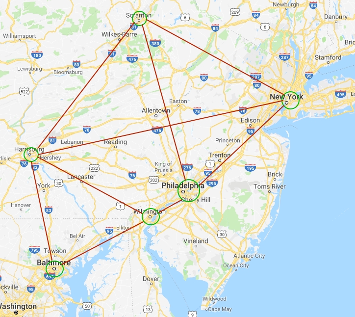
In this post, we will consider the following example of the graph: the cities are the vertices and the distances between them are the edges. You can see the Google Maps illustration of this structure in the figure below.
To start the work with the graph mentioned above, let’s launch Spark shell. To do this go to the Spark Home Directory and type in the console:
./bin/spark-shell
Now, we have to make some imports:
import org.apache.spark.graphx.Edgeimport org.apache.spark.graphx.Graphimport org.apache.spark.graphx.lib._
Creating the property graph
To create property graph we should firstly create an array of vertices and an array of edges. For vertices array, type in your spark shell:
val verArray = Array((1L, ("Philadelphia", 1580863)),(2L, ("Baltimore", 620961)), (3L, ("Harrisburg", 49528)),
 (4L, ("Wilmington", 70851)),
 (5L, ("New York", 8175133)),
 (6L, ("Scranton", 76089)))
The attributes of the vertices mean the city name and population, respectively.
As the output you will see the following:
verArray: Array[(Long, (String, Int))] = Array((1,(Philadelphia,1580863)), (2,(Baltimore,620961)), (3,(Harrisburg,49528)), (4,(Wilmington,70851)), (5,(New York,8175133)), (6,(Scranton,76089)))
To create edges array, type in the spark shell:
val edgeArray = Array(Edge(2L, 3L, 113),Edge(2L, 4L, 106), Edge(3L, 4L, 128),
 Edge(3L, 5L, 248),
 Edge(3L, 6L, 162),
 Edge(4L, 1L, 39),
 Edge(1L, 6L, 168),
 Edge(1L, 5L, 130),
 Edge(5L, 6L, 159))
The first and the second arguments indicate the source and the destination vertices identifiers and the third argument means the edge property which, in our case, is the distance between corresponding cities in kilometers.
The above-mentioned input will give us the following output:
edgeArray: Array[org.apache.spark.graphx.Edge[Int]] = Array(Edge(2,3,113), Edge(2,4,106), Edge(3,4,128), Edge(3,5,248), Edge(3,6,162), Edge(4,1,39), Edge(1,6,168), Edge(1,5,130), Edge(5,6,159))
Next, we will create RDDs from the vertices and edges arrays by using the sc.parallelize() command:
val verRDD = sc.parallelize(verArray)val edgeRDD = sc.parallelize(edgeArray)
We are ready to build a property graph. The basic property graph constructor takes an RDD of vertices and an RDD of edges and builds a graph.
val graph = Graph(verRDD, edgeRDD)
Now we have our property graph, and it is time to consider basic operations which can be performed with graphs such as filtration by vertices, filtration by edges, operations with triplets and aggregation.
Filtration by vertices
To illustrate the filtration by vertices let’s find the cities with population more than 50000. To implement this, we will use the filter operator:
graph.vertices.filter {    case (id, (city, population)) => population > 50000}.collect.foreach {     case (id, (city, population)) =>
     println(s"The population of $city is $population")
 }
And this is the result we get:
The population of Scranton is 76089The population of Wilmington is 70851The population of Philadelphia is 1580863 The population of New York is 8175133
 The population of Baltimore is 620961
Triplets
One of the core functionalities of GraphX is exposed through the triplets RDD. There is one triplet for each edge which contains information about both the vertices and the edge information. Let’s take a look through graph.triplets.collect.
As an example of working with triplets, we will find the distances between the connected cities:
for (triplet <- graph.triplets.collect) { println(s"""The distance between ${triplet.srcAttr._1} and ${triplet.dstAttr._1} is ${triplet.attr} kilometers""") }
As a result, you should see:
The distance between Baltimore and Harrisburg is 113 kilometersThe distance between Baltimore and Wilmington is 106 kilometersThe distance between Harrisburg and Wilmington is 128 kilometers The distance between Harrisburg and New York is 248 kilometers
 The distance between Harrisburg and Scranton is 162 kilometers
 The distance between Wilmington and Philadelphia is 39 kilometers
 The distance between Philadelphia and New York is 130 kilometers
 The distance between Philadelphia and Scranton is 168 kilometers
 The distance between New York and Scranton is 159 kilometers
Filtration by edges
Now, let’s consider another type of filtration, namely filtration by edges. For this purpose, we want to find the cities, the distance between which is less than 150 kilometers. If we type in the spark shell,
graph.edges.filter {  case Edge(city1, city2, distance) => distance < 150}.collect.foreach {   case Edge(city1, city2, distance) =>
   println(s"The distance between $city1 and $city2 is $distance")
 }
we will see the next result:
The distance between 2 and 3 is 113The distance between 2 and 4 is 106The distance between 3 and 4 is 128 The distance between 4 and 1 is 39
 The distance between 1 and 5 is 130
Aggregation
Another interesting task which can be considered here is aggregation. We will find total population of the neighboring cities. But before we start, we should change our graph a little. The reason for this is that GraphX deals only with directed graphs. But to take into account edges in both directions, we should add the reverse directions to the graph. Let’s take a union of reversed edges and original ones.
val undirectedEdgeRDD = graph.reverse.edges.union(graph.edges)val graph = Graph(verRDD, undirectedEdgeRDD)
Now we have an undirected graph with all the edges and directions taken into account, so we can perform the aggregation using aggregateMessages operator:
val neighbors = graph.aggregateMessages[Int](ectx => ectx.sendToSrc(ectx.dstAttr._2), _ + _)
To see the result, type:
neighbors.foreach(println(_))
You should get the following output,
(4,2251352)(1,8322073)(5,1706480) (2,120379)
 (6,9805524)
 (3,8943034)
where the first argument is the vertex id and the second argument is the total population of the neighboring cities.
Conclusions
GraphX is very useful Spark component which has many applications in different fields, from computer science to biology and social sciences. In this post, we have considered the simple graph example where the vertices are the cities and the edges are the distances between them. Some basic operations such as filtration by vertices, filtration by edges, operations with triplets and aggregation have been applied to this graph. All in all, we showed that Apache Spark GraphX component is very convenient and applicable for graph computations.

