The standard definition of a generalized Gaussian distribution can be found here. In this article, we explore a different type of generalized univariate normal distributions that satisfies useful statistical properties, with interesting applications. This new class of distributions is defined by its characteristic function, and applications are discussed in the last section. These distributions are semi-stable (we define what this means below). In short it is a much wider class than the stable distributions (the only stable distribution with a finite variance being the Gaussian one) and it encompasses all stable distributions as a subset. It is a sub-class of the divisible distributions. The distinctions are as follows:
- Stable distributions are jointly stable both under addition and multiplication by a scalar
- Semi-stable are separately stable under addition and multiplication by a scalar
- Divisible distributions are stable under addition
1. New two-parameter distribution G(a, b): introduction, properties
Semi-stable distributions can serve as a great introduction to explain the central limit theorem in a simple and elegant way. The family that we investigate here is governed by two parameters a and b. Distributions from that family are denoted as G(a, b). We focus exclusively on symmetrical distributions centered at zero.

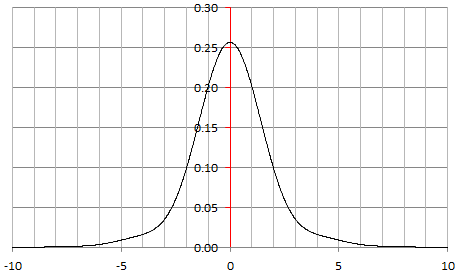
Figure 1: A special G(a, b) distribution, see section 4
By definition, they satisfy the following properties:
- If X is a random variable with a G(a, b) distribution and v is a real number, then vX has a G(av^β, bv) distribution.
- If X(1), …, X(n) are independently and identically distributed G(a, b), then X(1) + … + X(n) is G(na, b).
Here β ∈ [1, 2] is a fixed real number, not a parameter of the model. The notation v^β means v at power β. As a consequence, we have the following result.
2. Generalized central limit theorem

All these random variables have zero mean and are symmetrical. The case β = 2 corresponds to the standard central limit theorem. A fundamental consequence is that if β = 2, then G(a, 0) must be a Gaussian distribution. The notation Z ~ G(a,0) means that the distribution of Z is G(a, 0). The convergence is in distribution.
3. Characteristic function
The characteristic function ψ(t) of a random variable X uniquely defines its statistical distribution. We consider here CF’s that have the following form:

with the following requirements:
- a is strictly positive
- h is an even, real-valued function, thus h(t) = h(-t)
- h is bounded, and the minimum value of h is strictly above zero
- h is such that it yields a proper CF (one that is positive-definite, according to Bochner’s theorem)
In particular, if β = 1, we are dealing with generalized Cauchy distributions. Here we focus on β = 2, corresponding to generalized Gaussian distributions. If β = 2 and b = 0, then G(a, b) is Gaussian. If β = 1 and b = 0, then G(a, b) is Cauchy.
4. Density: special cases, moments, mathematical conjecture
The density is obtained by inverting the characteristic function, in other words, by computing its inverse Fourier transform. Since the density is also symmetrical and centered at zero, no complex numbers are involved, and it simplifies to

By construction, it always integrates to 1. If β = 1, none of the moments exist. If β is strictly between 1 and 2, the mean is zero but higher moments do not exist. If β = 2 (the case we are interested in) then all the moments exist, and all the odd moments are zero. If β > 2, it can not be a density.
The only thing that needs to be checked, to guarantee that we are dealing with a proper density, is that f must be positive everywhere. In order for this to be true, the function h must be carefully chosen. We are interested in the following special case exclusively:

Here α and λ are two fixed positive real numbers: just like β, they are not parameters of the model. Based on empirical evidence, I conjecture the following, assuming β = 2:
- If α > 2 and λ < 1, then the density is positive everywhere: it is a proper density
- If α > 4 and λ < 2, then the density is positive everywhere: it is a proper density
The density G(1, 1) corresponding to α = 2, β = 2, and λ = 1 is pictured in Figure 1. By contrast, if α = λ = β = 2, then f(13.56) = f(-13.56) = -0.000003388 is the absolute minimum for f. It is below zero, thus f is not a density.
All the moments can easily be derived from the characteristic function. Odd moments are zero, and for even moments, we have:

In particular, assuming β = 2, Var(X) = 2 α a. It does not depend on λ.
5. Simulations
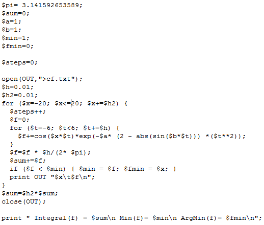
It is not easy to simulate deviates from G(a, b) using traditional methods based on the characteristic function, such as this one developed by Luc Devroye in 1980. I propose here a technique that I believe is simpler. First you need to compute the density function. The following program does that job:

You can download the source code here. It computes the density f(x) for 4,000 values of x equally spaced between -20 and +20. The next step is to compute the empirical cumulative distribution based on these 4,000 values: this is straightforward. Then you can use the classic inverse transform method, using the empirical inverse cumulative distribution, to generate the deviates in question.
Another way to simulate this type of distribution is to compute its moments (easy with Mathematica or WolframAlpha) using the formula at the bottom of section 4, see also here. Then use the Momentify R package, available here.
6. Weakly semi-stable distributions
The semi-stable distributions introduced here satisfy this property: if X(1), …, X(n) are independently and identically distributed G(a, b), then X(1) + … + X(n) is G(na, b). A weaker requirement would be that X(1) + X(2) is G(2a, b), resulting in a potentially larger class of distributions. Note that even with this weaker form, the generalized central limit theorem in section 2 may be preserved, unchanged.
We have:
- X(1) + X(2) is G(2a, b)
- G(2a, b) + G(2a, b) is G(4a, b)
- G(4a, b) + G(4a, b) is G(8a, b)
And so on. Let m = 2^n. Clearly, the main theorem in section 2 is preserved, unchanged, if you replace n by m. Thus if there is convergence, it must be for any n, not just for those that are are a power of 2. And the limiting distribution Z will also be G(a, 0).
7. Counter-example
Building distribution families that meet the requirements of section 1 is not that easy. We try here to build such distributions directly from the density rather than from the characteristic function, and we show that it does not work. The family in question is also governed by two parameters a and b with b > 0. These distributions are also symmetrical and centered at 0, and defined by the following density:

The characteristic function is as follows:

If X(1), X(2) are independently and identically distributed, from that same family of distributions, then
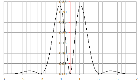
Clearly, the distribution of X(1) + X(2) can not belong to the same family as X, and thus we are dealing with a family of distributions that is not even weakly semi-stable. The distribution of X, with a = b = 1, is pictured below:

Figure 2: Counter-example
8. Applications and conclusions
Stable distributions with fat tails and infinite variance, such as Cauchy or Levy, have been used in financials models when the Gaussian law fails, see here. The class of distribution proposed here generalizes these stable distributions, yet still offers properties that make them easy to handle especially as far as the asymptotic behavior is concerned. The case β < 2 provides a fat tail and infinite variance. These distributions are also used in geopolitics, economics, and risk modeling: see here. The case β = 2 encompasses the Gaussian distribution, and yields a finite variance.
Likewise, divisible distributions such as Poisson have been used in a number of contexts. Most recently new divisible distributions were devised to model counts in data sets (see here.) Our class of semi-stable or weakly semi-stable distributions is more narrow but have nicer properties, making them good candidates when you need a distribution that has more stability than divisible distributions, and more flexible, more varied than stable distributions: in other words, something in between divisible and stable distributions, offering the best of both worlds.
Related article
- New Perspective on the Central Limit Theorem and Statistical Testing (also discussing stable distributions)
