The gradient descent algorithm is one of the most popular optimization techniques in machine learning. It comes in three flavors: batch or “vanilla” gradient descent (GD), stochastic gradient descent (SGD), and mini-batch gradient descent which differ in the amount of data used to compute the gradient of the loss function at each iteration.
The goal of this article is to describe the progress in the search for global optimizers based on Langevin Dynamics (LD), a modeling approach for molecular motion which has its origins on works by Albert Einstein and Paul Langevin on statistical mechanics in the early 1900s.
I will provide an elegant explanation, from the perspective of theoretical physics, to why variants of gradient descent are efficient global optimizers.
The Miracle Year
There was no sign that a revolution was about to happen. In 1904, had Albert Einstein abandoned physics, it is likely that his fellow scientists wouldn’t even have noticed. Fortunately, that didn’t happen. In 1905, the young patent clerk published four papers that revolutionized science.

Random Motion in a Fluid
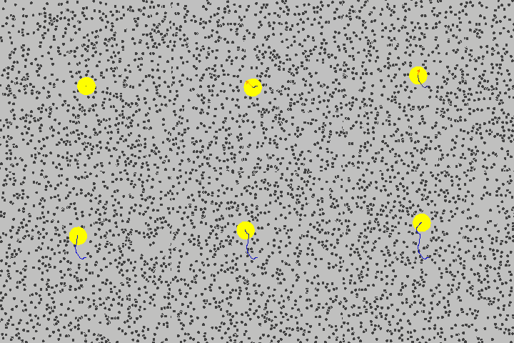
In one of those papers, Einstein derived a model for the so-called Brownian motion, the random motion of suspended particles in a liquid caused by collisions with smaller, fast-moving molecules (pollen grains moving in water for example). A dust particle colliding with gas molecules is shown in the figure below (source).

In this paper, he single-handedly confirmed the existence of atoms and molecules thus giving birth to a new branch of physics called molecular dynamics, and created a brand new field of applied mathematics known as stochastic calculus.
The Langevin Dynamics
In 1908, three years after Einstein published his landmark papers, the French physicist Paul Langevin published another groundbreaking article where he generalized Einstein’s theory and developed a new differential equation describing Brownian motion, known today as the Langevin Equation (LE)

where x is the position of the moving particle, m is its mass, R represents a (random) force generated by collisions with the smaller, fast-moving molecules of the fluid (see the animation above) and F represents any other external force. The random force R is a delta-correlated stationary Gaussian process with the following mean and variance:

where R is a normal process. The term “delta-correlated” means that the forces at two different times have zero correlation. The LE was the first mathematical equation describing thermodynamics out of equilibrium.

If the particle’s mass is small enough, we can set the left-hand side to zero. Furthermore, we can express a (conservative) force as the derivative of some potential energy. We obtain:

Langevin equation for small masses.
Now, writing

where δt is a small time interval, and moving terms around, we obtain the discretized Langevin equation for a particle with small mass:

Expressed this way, the Langevin equation describes incremental displacements of a particle undergoing Brownian motion.
A Short Interlude: a Python Code for Brownian Motion
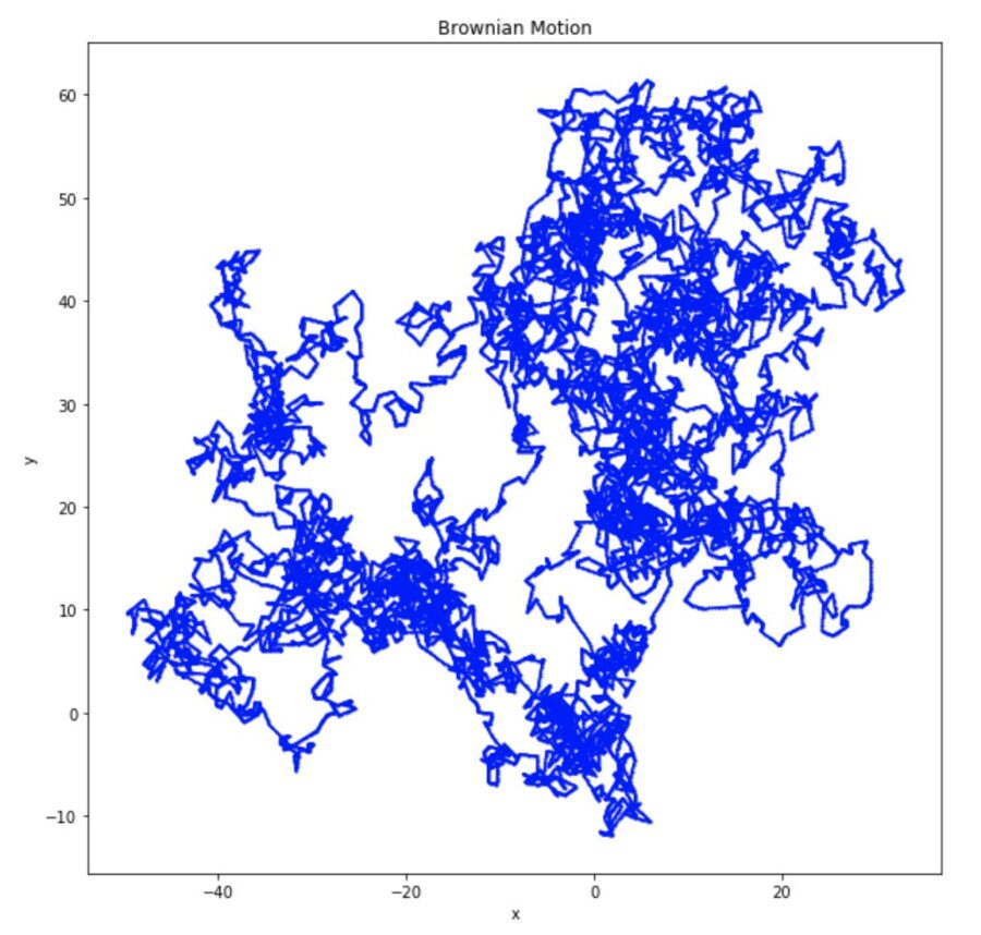
A Python implementation of Brownian motion can be found here. To simulate a 2D discrete Brownian process two 1D processes are used. The steps of the codes are:
- First, the number of time steps,
steps, is chosen. - The coordinates
xandyare cumulative sums of the random jumps (the functionnp.cumsum()is used to compute them) - The intermediary points
XandYare computed by interpolation usingnp.interp() - The motion is then plotted using the
plot()function
The code is:
import numpy as np
import matplotlib.pyplot as plt
%matplotlib inline
steps = 5000
random.seed(42)
x,y = np.cumsum(np.random.randn(steps)), np.cumsum(np.random.randn(steps))
points = 10
ip = lambda x, steps, points: np.interp(np.arange(steps*points),
np.arange(steps)*points,
 x)
 X, Y = ip(x, steps, points), ip(y, steps, points)
fig, ax = plt.subplots(1, 1, figsize=(10, 10))
ax.set_title('Brownian Motion')
ax.set_xlabel('x')
 ax.set_ylabel('y')
 ax.plot(X, Y, color='blue',
 marker='o',  markersize=1)

Langevin Dynamics and Global Minima
An important property of Langevin dynamics is that the diffusion distribution p(x) of the stochastic process x(t) (where x(t) obeys the Langevin equation given above) converges to a stationary distribution, the ubiquitous Boltzmann distribution (BD)

which concentrates around the global minimum of the potential energy E(x) (from its functional form, we can easily see that the BD peaks on the global minimum of the potential energy E(x)). More precisely, as shown by Hajekand others, if the temperature is slowly decreased to zero following the discrete steps:

then p(x) will converge to the Boltzmann distribution for large values of n (and x will converge to the global minimum of E(x)). The Langevin equation for time-dependent temperatures is usually interpreted as describing the decay of metastable physical states into the ground state of the system (which is the global minimum of the energy). One can, therefore, use Langevin dynamics to design algorithms that are global minimizers even of potential non-convex function.
This principle is the basis of the simulated annealing technique, used for obtaining the approximate global optimum of functions.

Gradient Descent Algorithms
I will now switch gears to machine learning optimization algorithms.
Gradient descent is a simple iterative optimization algorithm for minimizing (or maximizing) functions. In the context of machine learning, these functions are the loss functions (or cost functions). For concreteness, consider a multivariate loss function L(w) defined for all points w around some fixed point p. The GD algorithm is based on the simple property that starting at any point p the function L(w) decreases fastest in the direction of its negative gradient:

One starts by guessing an initial value for the (unknown) minimum and computes the sequence

following the iterative process

where γ is the learning rate, which is allowed to change at each iteration n. If the loss function L and its gradient have certain properties and the learning rate variation is chosen following certain protocols, local convergence is guaranteed (convergence to a global minimum is guaranteed only if L is convex since for convex functions any local minimum is also a global one).
Stochastic Gradient Descent (SGD) and Mini-Batch Gradient Descent
In contrast to the basic GD algorithm, which scans the full dataset at each iteration, SGD and mini-batch GD uses only a subset of the training data. SGD uses a single sample of the training data to update the gradient in each iteration i.e. as it sweeps through the training data, it performs the above update of w for each training example. Mini-batch GD performs parameter updates using mini-batches of training examples.
Let us put this in mathematical terms. For a general training set with n samples,

the loss function has the general form:

In the case of mini-batch gradient descent, the sum is only over the training examples inside the batch. SGD, in particular, uses one sample only. These procedures have two main advantages versus vanilla GD: they are much faster and can handle datasets that are much larger (since they use either one or a few samples).
Defining G and g as indicated below, we have in this case:

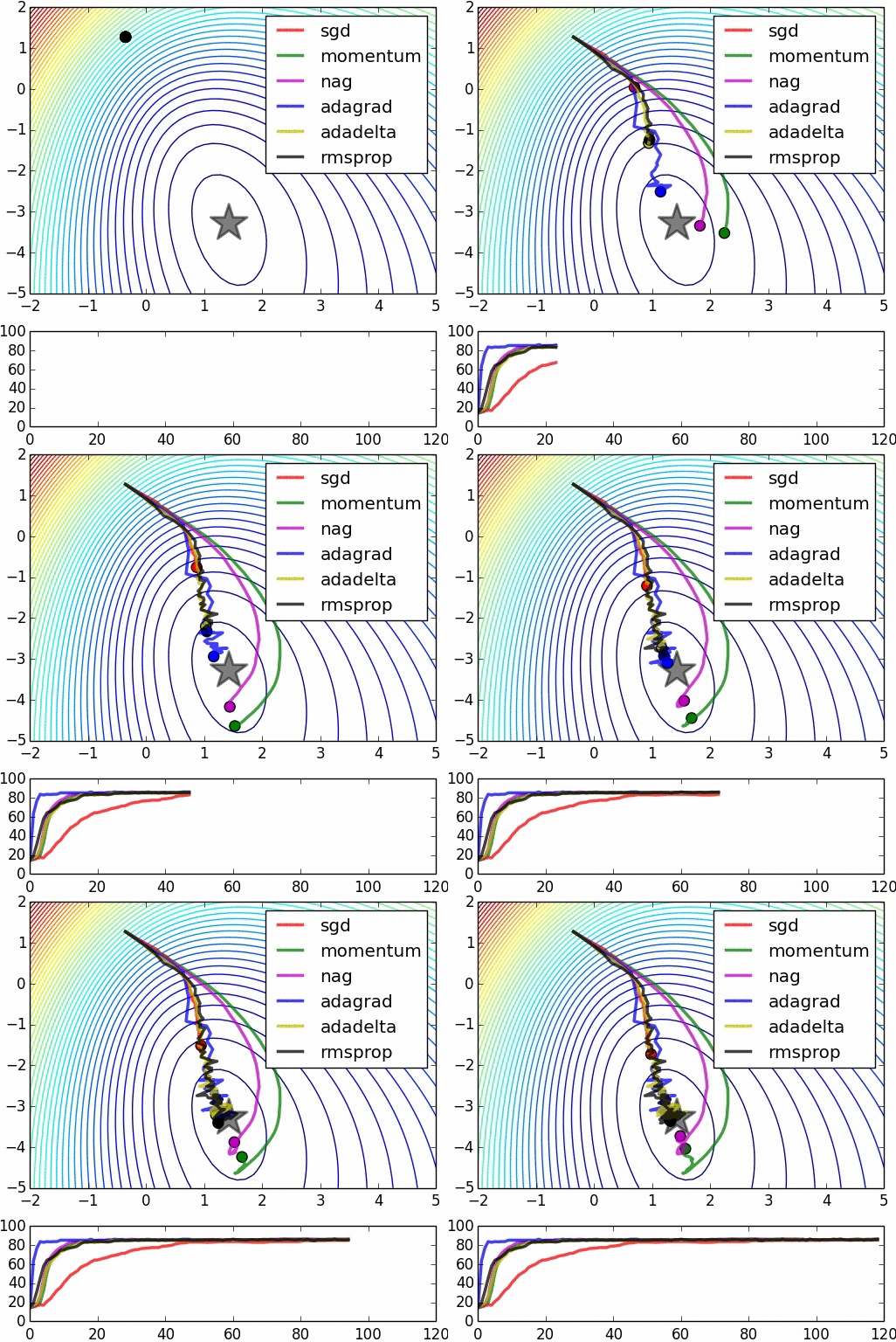
In the great animation below by Alec Radford, the SGD convergence is shown together with other methods (these other methods, not mentioned in this article, are more recent improvements of SGD).

Machine Learning and Physics: Gradient Descent as a Langevin Process
The next (and last) step is crucial for the argument. I omitted more rigorous aspects for the main idea to come across.
We can write the mini-batch gradient as a sum between the full gradient and a normally distributed η:

Now substituting this expression in the GD iteration expression we obtain:

An Elegant Link
Comparing the expression for the mini-batch gradient descent iteration with the Langevin equation we can immediately notice their similarity. More precisely, they become identical using the following correspondence:

Substituting δt by γ in the second expression we find that

SGD or mini-batch gradient descent algorithms are therefore formally analogous to Langevin processes and that explains why, provided the learning rate is varied following the previously mentioned protocols, they have a very high probability of selecting global minima.
This result is far from new. There are in fact many proofs that the addition of a noise term to the usual gradient descent recursion makes the algorithm converge to global minima. It must be emphasized that it is the “cooling protocol” of the learning rate that provides the crucial “extra” randomization that allows the algorithm to escape local minima and converge to the global one.
Conclusion
In this article, I showed that by thinking of either stochastic or mini-batch gradient descent as Langevin stochastic processes (with energy identified with the loss function) and including an extra level of randomization via the learning rate, we can understand why these algorithms can work so well as global optimizers. It is an elegant result which shows that examining a problem from multiple viewpoints is often extremely useful.
Thanks for reading!
My Github and my personal website www.marcotavora.me have (hopefully) some other interesting stuff both about data science and physics.
As always, constructive criticism and feedback are welcome!
This article was originally published on Towards Data Science.
