What are the Learning Rules in Neural Network?
Learning rule or Learning process is a method or a mathematical logic. It improves the Artificial Neural Network’s performance and applies this rule over the network. Thus learning rules updates the weights and bias levels of a network when a network simulates in a specific data environment.
Applying learning rule is an iterative process. It helps a neural network to learn from the existing conditions and improve its performance.
Let us see different learning rules in the Neural network:
- Hebbian learning rule – It identifies, how to modify the weights of nodes of a network.
- Perceptron learning rule – Network starts its learning by assigning a random value to each weight.
- Delta learning rule – Modification in sympatric weight of a node is equal to the multiplication of error and the input.
- Correlation learning rule – The correlation rule is the supervised learning.
- Outstar learning rule – We can use it when it assumes that nodes or neurons in a network arranged in a layer.
1. Hebbian Learning Rule
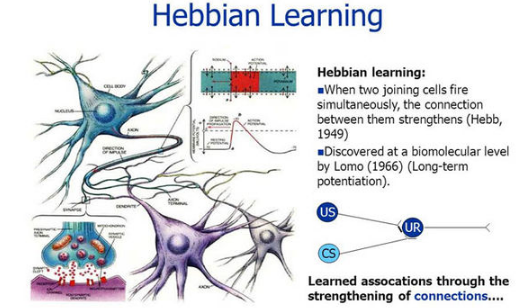
The Hebbian rule was the first learning rule. In 1949 Donald Hebb developed it as learning algorithm of the unsupervised neural network. We can use it to identify how to improve the weights of nodes of a network.
The Hebb learning rule assumes that – If two neighbor neurons activated and deactivated at the same time. Then the weight connecting these neurons should increase. For neurons operating in the opposite phase, the weight between them should decrease. If there is no signal correlation, the weight should not change.
When inputs of both the nodes are either positive or negative, then a strong positive weight exists between the nodes. If the input of a node is positive and negative for other, a strong negative weight exists between the nodes.
At the start, values of all weights are set to zero. This learning rule can be used0 for both soft- and hard-activation functions. Since desired responses of neurons are not used in the learning procedure, this is the unsupervised learning rule. The absolute values of the weights are usually proportional to the learning time, which is undesired.
The Hebbian learning rule describes the formula as follows:
2. Perceptron Learning Rule
As you know, each connection in a neural network has an associated weight, which changes in the course of learning. According to it, an example of supervised learning, the network starts its learning by assigning a random value to each weight.
Calculate the output value on the basis of a set of records for which we can know the expected output value. This is the learning sample that indicates the entire definition. As a result, it is called a learning sample.
The network then compares the calculated output value with the expected value. Next calculates an error function ∈, which can be the sum of squares of the errors occurring for each individual in the learning sample.
Computed as follows:
Perform the first summation on the individuals of the learning set, and perform the second summation on the output units. Eij and Oij are the expected and obtained values of the jth unit for the ith individual.
The network then adjusts the weights of the different units, checking each time to see if the error function has increased or decreased. As in a conventional regression, this is a matter of solving a problem of least squares.
Since assigning the weights of nodes according to users, it is an example of supervised learning.


