Section 3 was added on October 11. Section 4 was added on October 19. A $2,000 award is offered to solve any of the open questions, click here for details.
This is another off-the-beaten-path problem, one that you won’t find in textbooks. You can solve it using data science methods (my approach) but the mathematician with some spare time could find an elegant solution. Share it with your colleagues to see how math-savvy they are, or with your students. I was able to make substantial progress in 1-2 hours of work using Excel alone, thought I haven’t found a final solution yet (maybe you will.) My Excel spreadsheet with all computations is accessible from this article. You don’t need a deep statistical background to quickly discover some fun and interesting results playing with this stuff. Computer scientists, software engineers, quants, BI and analytic professionals from beginners to veterans, will also be able to enjoy it!
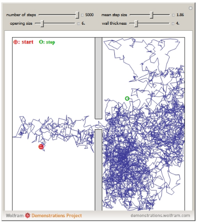
Source for picture: 2-D constrained random walk (snapshot – video available here)
1, The problem
We are dealing with a stochastic process barely more complicated than a random walk. Random walks are also called drunken walks, as they represent the path of a drunken guy moving left and right seemingly randomly, and getting lost over time. Here the process is called self-correcting random walk or also reflective random walk, and is related to controlled random walks, and constrained random walks (see also here) in the sense that the walker, less drunk than in a random walk, is able to correct any departure from a straight path, more and more over time, by either slightly over- or under-correcting at each step. One of the two model parameters (the positive parameter a) represents how drunk the walker is, with a = 0 being the worst. Unless a = 0, the amplitude of the corrections decreases over time to the point that eventually (after many steps) the walker walks almost straight and arrives at his destination. This model represents many physical processes, for instance the behavior of a stock market somewhat controlled by a government to avoid bubbles and implosions, or when it hits a symbolic threshold and has a hard time breaking through. It is defined as follows:
Let’s start with X(1) = 0, and define X(k) recursively as follows, for k > 1:
and let’s define U(k), Z(k), and Z as follows:
where the V(k)’s are deviates from independent uniform variables on [0, 1], obtained for instance using the function RAND in Excel. So there are two positive parameters in this problem, a and b, and U(k) is always between 0 and 1. When b = 1, the U(k)’s are just standard uniform deviates, and if b = 0, then U(k) = 1. The case a = b = 0 is degenerate and should be ignored. The case a > 0 and b = 0 is of special interest, and it is a number theory problem in itself, related to this problem when a = 1. Also, just like in random walks or Markov chains, the X(k)’s are not independent; they are indeed highly auto-correlated.
Prove that if a < 1, then X(k) converges to 0 as k increases. Under the same condition, prove that the limiting distribution Z
- always exists, (Note: if a > 1, X(k) may not converge to zero, causing a drift and asymmetry)
- always takes values between -1 and +1, with min(Z) = -1 and max(Z) = +1,
- is symmetric, with mean and median equal to 0
- and does not depend on a, but only on b.
For instance, for b =1, even a = 0 yields the same triangular distribution for Z, as any a > 0.
If a < 1 and b = 0, (the non-stochastic case) prove that
- Z can only take 3 values: -1 with probability 0.25, +1 with probability 0.25, and 0 with probability 0.50
- If U(k) and U(k+1) have the same sign,then U(k+2) is of opposite sign
And here is a more challenging question: In general, what is the limiting distribution of Z? Also, what happens if you replace the U(k)’s with (say) Gaussian deviates? Or with U(k) = | sin (k*k) | which has a somewhat random behavior?
2. Hints to solve this problem
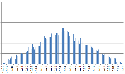
It is necessary to use a decent random number generator to perform simulations. Even with Excel, plotting the empirical distribution of Z(k) for large values of k, and matching the kurtosis, variance and empirical percentiles with those of known statistical distributions, one quickly notices that when b = 1 (and even if a = 0) the limiting distribution Z is well approximated by a symmetric triangular distribution on [-1, 1], and thus centered on 0, with a kurtosis of -3/5 and and a variance of 1/6. In short, this is the distribution of the difference of two uniform random variables on [0, 1]. In other words, it is the distribution of U(3) – U(2). Of course, this needs to be proved rigorously. Note that the limiting distribution Z can be estimated by computing the values Z(n+1), …, Z(n+m) for large values of n and m, using just one instance of this simulated stochastic process.
Does it generalize to other values of b? That is, does Z always have the distribution of U(3) – U(2)? Obviously not for the case b = 0. But it could be a function, combination and/or mixture of U(3), –U(2), and U(3) – U(2). This works both for b = 0 and b = 1.
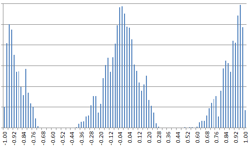
Figure 1: Mixture-like distribution of Z (estimated) when b = 0.01 and a = 0.8
Interestingly, for small values of b, the limiting distribution Z looks like a mixture of (barely overlapping) simple distributions. So it could be used as a statistical model in clustering problems, each component of the mixture representing a cluster. See Figure 1.
Figure 2: Triangular distribution of Z (estimated) when b = 1 and a = 0.8
The spreadsheet with all computations and model fitting can be downloaded here..
3. Deeper dive
So far, my approach has been data science oriented: it looks more like a guesswork. Here I switch to mathematics, to try to derive the distribution of Z. Since it does not depend on the parameter a, let us assume here that a = 0. Note that when a = 0, X(k) does not converge to zero; instead X(k) = Z(k) and both converge in distribution to Z. It is obvious that X(k) is a mixture of distributions, namely X(k-1) + U(k) and X(k-1) – U(k). Since X(k-1) is in turn a mixture, X(k) is actually a mixture of mixtures, and so on, In short, it has the distribution of some nested mixtures.
As a starting point, it would be interesting to study the variance of Z (the expectation of Z is equal to 0.) The following formula is incredibly accurate for any value of b between 0 and 1, and even beyond. It is probably an exact formula, not an approximation. It was derived using the tentative density function obtained at the bottom of this section, for Z:
It is possible to obtain a functional equation for the distribution P(Z < z), using the equations that define X(k) in section 1, with a = 0, and letting k tends to infinity. It starts with
Let’s introduce U as a random variable with the same distribution as U(k) or U(2). As k tends to infinity, and separating the two cases x negative and x positive, we get
Taking advantages of symmetries, this can be further simplified to
where F represents the distribution function, f represents the density function, and U has the same distribution as U(2), that is
Taking the derivative with respect to z, the functional equation becomes the following Fredholm integral equation, the unknown being Z‘s density function:
We have the following particular cases:
- When b tends to zero, the distribution of Z converges to a uniform law on [-1, 1] thus with a variance equal to 1/3.
- When b = 1/2, Z has a parabolic distribution on [-1, +1], defined by P(Z < z) = (2 + 3z – z^3)/4. This needs to be proved, for instance by plugging this parabolic distribution in the functional equation, and checking that the functional equation is verified if b = 1/2. However, a constructive proof would be far more interesting.
- When b = 1, Z has the triangular distribution discussed earlier. The density function for Z, defined as the derivative of P(Z < z) with respect to z, is equal to 1 – |z| when b = 1, and 3 (1 – z^2) / 4 when b = 1/2.
So for b = 1, b = 1/2, or the limiting case b = 0, we have the following density for Z, defined on [-1, 1]:
Is this formula valid for any b between 0 and 1? This is still an open question. The functional equation applies regardless of U‘s distribution though, even if exponential or Gaussian. The complexity in the cases discussed here, arises from the fact that U‘s density is not smooth enough, due to its bounded support domain [0, 1] (outside the support domain, the density is equal to 0.) A potential more generic version of the previous formula would be:
where E denotes the expectation. However, I haven’t checked whether and under which conditions this formula is correct or not, except for the particular cases of U discussed here. One of the requirements is that the support domain for U is [0, 1]. If this formula is not exact in general, it might still be a good approximation in some cases.
4. Potential Areas of Research
Here are a few interesting topics for research:
- Develop a 2-D or 3-D version of this process, investigate potential applications in thermodynamics or statistical mechanics, for instance modeling movements of gas molecules in a cube as the temperature goes down (a >0) or is constant (a = 0), and comparison with other stochastic processes used in similar contexts..
- Continuous version of the discrete reflective random walk investigated here, with a = 0, and increments X(k) – X(k-1) being infinitesimally small, following a Gaussian rather than uniform distribution. The limiting un-constrained case is known as a Wiener process or Brownian motion. What happens if this process is also constrained to lie between -1 and +1 on the Y-axis? This would define a reflected Wiener process, see also here for a similar process, and also here.
- Another direction is to consider the one-dimensional process as time series (which economists do) and to study the multivariate case, with multiple cross-correlated time series.
- For the data scientist, it would be worth checking whether and when, based on cross-validation, my process provides better model fitting, leading to more accurate predictions and thus better stock trading ROI (than say a random walk, after removing any trend or drift) when applied to real stock market data publicly available.
This is the kind of mathematics used by Wall Street quants and in operations research. Hopefully my presentation here is much less arcane than the traditional literature on the subject, and accessible to a much broader audience, even though it features the complex equations characterizing such a process (and even hinting to a mathematical proof that is not as difficult as it might seem at first glance, and supported by simulations). Note that my reflective random walk is not a true random walk in the classical sense of the term: A better term might be more appropriate.
5. Solution for the (non-stochastic) case b = 0
Andrei Chtcheprov submitted the following statements, with proof :
- If a < = 1, then the sequence {X(k)} converges to zero.
- If a = 3, {X(k)} converges to Zeta(3) – 5/4 =~ -0.048.
- If a = 4, {X(k)} converges to (Pi^4 / 90) – 9/8 =~ -0.043.
You can read his proof here. Much more can also be explored regarding the case b = 0. For instance, when a = 1 and b = 0, the problem is similar to this one, where we try to approximate the number 2 by converging sums of elementary positive fractions without ever crossing the boundary Y= 2, staying below at all times. Here, by contrast, we try to approximate 0, also by converging sums of the same elementary fractions, but allowing each term to be either positive or negative, thus crossing the boundary Y = 0 very regularly. The alternance of the signs for X(k), is a problem of interest: It shows strong patterns.
To include mathematical formulas in this article, I used this app. Those interested in winning the award by offering a theoretical solution should read this article, where I solved another stochastic integral equation of similar complexity (with mathematical proof), in a related context (chaotic systems.)
For related articles from the same author, click here or visit www.VincentGranville.com. Follow me on LinkedIn.
DSC Resources
- Services: Hire a Data Scientist | Search DSC | Classifieds | Find a Job
- Contributors: Post a Blog | Ask a Question
- Follow us: @DataScienceCtrl | @AnalyticBridge
Popular Articles


