Identifying Traffic Signs with Deep Learning

Successful detection and classification of traffic signs is one of the important problem to be solved if we want self driving cars. Idea is to make automobiles smart enough so as to achieve least human interaction for successful automation. Swift rise in dominance of deep learning over classical machine learning methods which is complemented by advancement in GPU (Graphics Processing Unit) has been astonishing in fields related to image recognition, NLP, self-driving cars etc.

Deep Learning

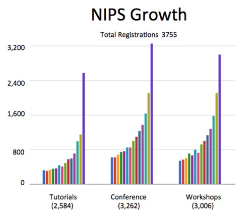
The chart only goes to 2015 and 2016 NIPS had over 6,000 attendees. Chart displays surge in interest in deep learning and related techniques.

Deep learning is a class of machine learning technique where artificial neural network uses multiple hidden layers. Lot of credit goes to David Hubel and Torsten Wiesel, two famous neurophysiologists, who showed how neurons in the visual cortex work. Their work determined how neurons with similar functions are organized into columns, tiny computational machines that relay information to a higher region of the brain, where visual image is progressively formed.

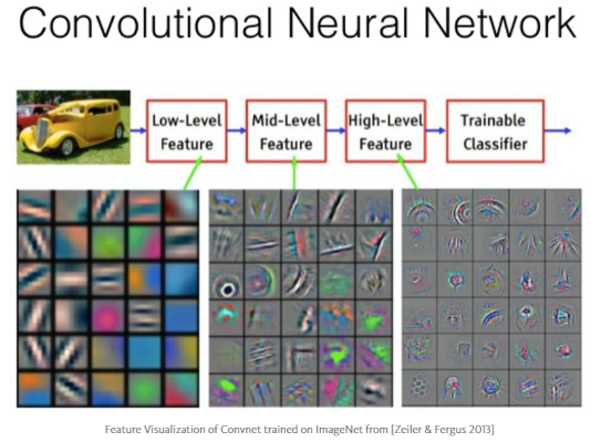
In layman’s term brain combines low level features such as basic shapes, curves and builds more complex shapes out of it. A deep convolutional neural network is similar. It first identifies low level features and then learns to recognize and combines these features to learn more complicated patterns. These different levels of features come from different layers of the network.

Lets see how simple deep convolution neural network performs on traffic sign dataset.

Model Architecture and Hyper parameters

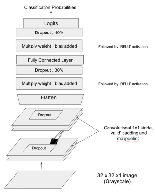
Tensorflowis used to implement deep conv net for traffic sign classification. RELU was used for activation to introduce non linearity and drop out of varying percentages was used to avoid overfitting at different stages. It was hard to believe that simple deep net was able to achieve high accuracy on the training data. Following is the architecture used for traffic sign classification.

def deepnn_model(x,train=True):

  # Arguments used for tf.truncated_normal, randomly defines variables for the weights and biases for each layer

  x = tf.nn.conv2d(x, layer1_weight, strides=[1, 1, 1, 1], padding=’VALID’)

  x = tf.nn.bias_add(x, layer1_bias)

  x = tf.nn.relu(x)

  x = tf.nn.max_pool(x,ksize=[1, 2, 2, 1],strides=[1, 2, 2, 1],padding=’SAME’)

  if(train):

    x = tf.nn.dropout(x, dropout1)

  x = tf.nn.conv2d(x, layer2_weight, strides=[1, 1, 1, 1], padding=’VALID’)

  x = tf.nn.bias_add(x, layer2_bias)

  x = tf.nn.relu(x)

  conv2 = tf.nn.max_pool(x,ksize=[1, 2, 2, 1],strides=[1, 2, 2, 1],padding=’SAME’)

  if(train):

    conv2 = tf.nn.dropout(conv2, dropout2)

  fc0 = flatten(conv2)

  fc1 = tf.add(tf.matmul(fc0, flat_weight),bias_flat)

  fc1 = tf.nn.relu(fc1)

  if(train):

    fc1 = tf.nn.dropout(fc1, dropout3)

  fc1 = tf.add(tf.matmul(fc1, flat_weight2),bias_flat2)

  fc1 = tf.nn.relu(fc1)

  if(train):

    fc1 = tf.nn.dropout(fc1, dropout4)

  fc1 = tf.add(tf.matmul(fc1, flat_weight3),bias_flat3)

  logits = tf.nn.relu(fc1)

  return logits

Result

My aim was to achieve 90 percent accuracy to start with simple architecture and I was surprised to see it close to 94 percent in the first run. Further adding more layers and complexity into the model complemented by data augmentation can achieve accuracy as high as 98 percent.