I recently created a ‘particle optimizer’ and published a pip python package called kernelml. The motivation for making this algorithm was to give analysts and data scientists a generalized machine learning algorithm for complex loss functions and non-linear coefficients. The optimizer uses a combination of simple machine learning and probabilistic simulations to search for optimal parameters using a loss function, input and output matrices, and (optionally) a random sampler. I am currently working more features and hope to eventually make the project open source.
Example use case:
Lets take the problem of clustering longitude and latitude coordinates. Clustering methods such as K-means use Euclidean distances to compare observations. However, The Euclidean distances between the longitude and latitude data points do not map directly to Haversine distance. That means if you normalize the coordinate between 0 and 1, the distance won’t be accurately represented in the clustering model. A possible solution is to find a projection for latitude and longitude so that the Haversian distance to the centroid of the data points is equal to that of the projected latitude and longitude in Euclidean space.

The result of this coordinate transformations allows you represent the Haversine distance, relative to the center, as Euclidean distance, which can be scaled and used in a cluster solution.
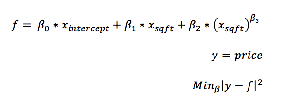
Another, simpler problem is to find the optimal values of non-linear coefficients, i.e, power transformations in a least squares linear model. The reason for doing this is simple: integer power transformations rarely capture the best fitting transformation. By allowing the power transformation to be any real number, the accuracy will improve and the model will generalize to the validation data better.

To clarify what is meant by a power transformation, the formula for the model is provided above.
The algorithm:
The idea behind kernelml is simple. Use the parameter update history in a machine learning model to decide how to update the next parameter set. Using a machine learning model as in the backend causes a bias variance problem, specifically, the parameter updates become more biased each iteration. The problem can be solved by including a monte carlo simulation around the best recorded parameter set after each iteration.
The issue of convergence:
The model saves the best parameter and user-defined loss after each iteration. The model also record a history of all parameter updates. The question is how to use this data to define convergence. One possible solution is:
convergence = (best_parameter-np.mean(param_by_iter[-10:,:],axis=0))/(np.std(param_by_iter[-10:,:],axis=0))
if np.all(np.abs(convergence)<1):
print(‘converged’)
break
The formula creates a Z-score using the last 10 parameters and the best parameter. If the Z-score for all the parameters is less than 1, then the algorithm can be said to have converged. This convergence solution works well when there is a theoretical best parameter set. This is a problem when using the algorithm for clustering. See the example below.
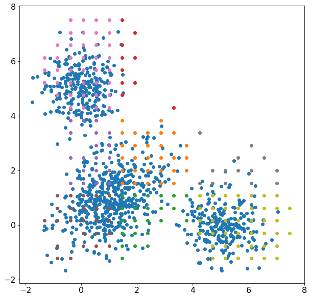
 Figure 1: Clustering with kernelml, 2-D multivariate normal distribution (blue), cluster solution (other colors)
We won’t get into the quality of the cluster solution because it is clearly not representative of the data. The cluster solution minimized the difference between a multidimensional histogram and the average probability of 6 normal distributions, 3 for each axis. Here, The distributions can ‘trade’ data points pretty easily which could increase convergence time. Why not just fit 3 multivariate normal distributions? There is a problem with simulating the distribution parameters because some parameters have constraints. The covariance matrix needs to be positive, semi-definite, and the inverse needs to exist. The standard deviation in a normal distribution must be >0. The solution used in this model incorporates the parameter constraints by making a custom simulation for each individual parameter. I’m still looking for a good formulation for how to efficiently simulate the covariance matrix for a multivariate normal distribution.
Why use kernelml instead of Expectation Maximization?
A non-normal distribution, such as Poisson, might not fit well with other dimensions in a multivariate normal cluster solution. In addition, as the number of dimensions increases, the probability that one cluster has a feature that only has non-zero values also increases. This poses a problem for the EM algorithm as it tries to update the covariation matrix. The covariance between the unique feature and other dimensions will be zero, or the probability that another cluster will accept an observation with this non-zero value is zero.
Probabilistic optimizer benefits:
The probabilistic simulation of parameters has some great benefits over fully parameterized models. First, regularization is included in the prior random simulation. For example, if prior random simulation of is between -1 and 1, it can be reasoned that the parameters will update with equal importance. In addition, while the algorithm is converging, each iteration produces a set of parameters that samples around the global, or local, minimum loss. There are two main benefits of this: 1) a confidence interval can be established for each parameter 2) the predicted output from each parameter set can be a useful feature in a unifying model.
The code for the clustering example, other uses cases, and documentation (still in progress) can be found in github.
