Finding and Fixing Autocorrelation

Autocorrelation can ruin your regression analysis.
How to spot autocorrelation in your data with visual tools and formal tests.
Tips to remove autocorrelation.

Autocorrelation is a measure of similarity (correlation) between adjacent data points; It is where data points are affected by the values of points that came before. Informally, it is the degree to which two observations compare as a function of the time-lapse between observations [1]. Recognizing autocorrelation in your data and fixing the problem is vital if you are to trust the results of your regression or other analysis. This is because autocorrelation can cause problems like:

One or more regression coefficients falsely reported as statistically significant.
Faux correlations between variables on inferential statistical tests [2].
T-statistics that are too large.
Ordinary Least Squares standard errors and test statistics that are not valid [3].

Why does autocorrelation happen?

Autocorrelation has a wide range of causes. These include carryover effect, where effects from a prior test or event affect results. For example, expenditures in a particular category are influenced by the same category of expenditure from the preceding time-period. Another common cause of autocorrelation is the cumulative impact of removing variables from a regression equation. The introduction of autocorrelation into data might also be caused by incorrectly defining a relationship, or model misspecification. For example, you might think there is a linear relationship between predictors and responses when in fact there is a log or exponential factor in the model [1].

In many circumstances, autocorrelation cant be avoided; This is especially true of many natural processes including some behavior of animals, bacteria [2], and viruses [1]. When working with time-series data, time itself causes self-correlation.[1].

Detecting autocorrelation

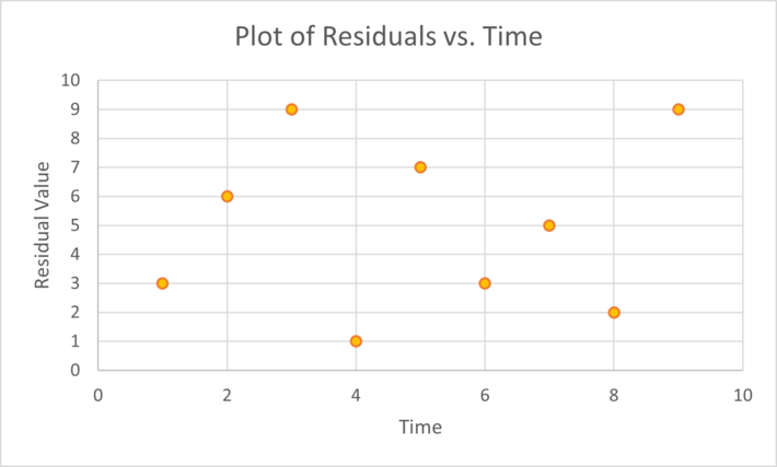
One of the easiest ways to spot dependency is to create a scatterplot of residuals vs. time for an observation (assuming your data is ordered by time). Randomly scattered data indicates no dependency, but if there is a noticeable pattern, your data probably has dependency issue [5]. The following chart shows a random pattern, suggesting no autocorrelation:

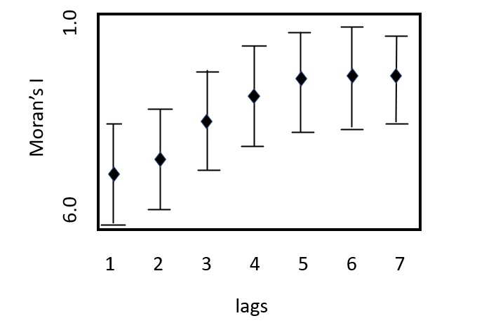
You can also make a correlogram [7], which is sometimes combined with a measure of correlation like Morans I.

A correlogram showing a consistent upward trend and high Morans I values: indicators of serial correlation.

As serial correlation invalidates many hypothesis tests and standard errors, you may want to run a more formal test for it.

The Durbin Watson test is the traditional go to to test for AR(1) serial correlationthe simplest type of structure where autocorrelation might occur. A rule of thumb is that DW-test statistic values outside of the range of 1.5 to 2.5 may be cause for concern; Values lower than 1 or more than 3 are a moderate to high cause for concern [6]. The DW test has a few stumbling blocks:

Critical values are found in a table, which can be cumbersome,
The test may be inconclusive unless very clear autocorrelations are identified,
It cannot be run on a model with a constant term.

The DW test will also not work with a lagged dependent variableuse Durbins h statistic instead. Other tests for autocorrelation include the Breusch-Godfrey Lagrange multiplier testa more general test for higher order autocorrelations, and the Ljung Box test, which tests whether observations are random and independent over time.

Tips for Fixing Autocorrelation

The first step to fixing time-dependency issues is usually to identify omission of a key predictor variable in your analysis. Next, check to make sure you havent misspecified your modelfor example, you may have modeled a linear relationship as exponential. If these steps dont fix the problem, consider transforming the variables. Popular methods are:

Cochrane-Orcutt: This is an iterative process. This basic approach does have a few issues: it does not always work, especially when errors are positively autocorrelated. In addition, the first sample is discarded during transformation, which is an issue for small samples. The Prais-Winsten method is an alternative that retains the first sample with appropriate scaling [10].
Hildreth-Lu: A non-iterative alternative which is similar to Box-Cox transformation.

DSCs Vincent Granville [11] offers a radically different and simpler approach to the usual methods: randomly re-shuffle the observations. If this doesnt fix the issue, this indicates there is something fundamentally wrong about the data set, perhaps with the way the data was collected. In most cases, this approach should work. If it doesnt, cleaning the data may help or in extreme casesthrow out the data and start over.