Dogs vs. Cats: Image Classification with Deep Learning using TensorFlow in Python

The problem

Given a set of labeled images of  cats and dogs, a  machine learning model  is to be learnt and later it is to be used to classify a set of new images as cats or dogs. 

• The original dataset contains a huge number of images, only a few sample images are chosen (1100 labeled images for cat/dog as training and 1000images from the test dataset) from the dataset, just for the sake of  quick demonstration of how to solve this problem using deep learning (motivated by the Udacity course Deep Learning by Google), which is going to be described (along with the results) in this article.

• The accuracy on the test dataset is not going to be good in general for the above-mentioned reason. In order to obtain good accuracy  on the test dataset using deep learning, we need to train the models with a large number of input images (e.g., with all the training images from the kaggle dataset).
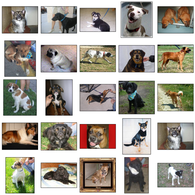
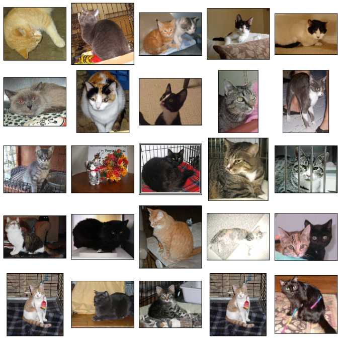
• A few sample labeled images from the training dataset are shown below.

Dogs

Cats
As a pre-processing step, all the images are first resized to 50×50 pixel images.

Classification with a few off-the-self classifiers

• First, each image from the training dataset is fattened and represented as 2500-length vectors (one for each channel).

• Next, a few sklearn models are trained on this flattened data. Here are the results

As shown above, the test accuracy is quite poor with a few sophisticated off-the-self classifiers.

Classifying images using Deep Learning with Tensorflow

Now let’s first train a logistic regression and then a couple of neural network models by introducing L2 regularization for both the models.

• First, all the images are converted to gray-scale images.
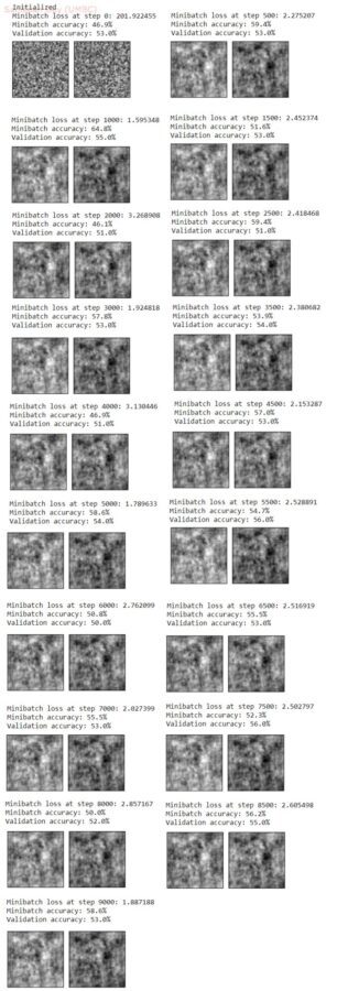
• The following figures visualize the weights learnt for the cat vs. the dog class during training the logistic regression  model with SGD with L2-regularization (λ=0.1, batch size=128).https://sandipanweb.files.wordpress.com/2017/08/cd_nn_no_hidden.png… 43w” sizes=”(max-width: 224px) 100vw, 224px” />

Test accuracy: 53.6% 

• The following animation visualizes the weights learnt for 400 randomly selected hidden units using a neural net with a single hidden layer with 4096 hidden nodes by training the neural net model  with SGD with L2-regularization (λ1=λ2=0.05, batch size=128).

  Minibatch loss at step 0: 198140.156250
  Minibatch accuracy: 50.0%
  Validation accuracy: 50.0%

  Minibatch loss at step 500: 0.542070
  Minibatch accuracy: 89.8%
  Validation accuracy: 57.0%

  Minibatch loss at step 1000: 0.474844
  Minibatch accuracy: 96.9%
  Validation accuracy: 60.0%

  Minibatch loss at step 1500: 0.571939
  Minibatch accuracy: 85.9%
  Validation accuracy: 56.0%

  Minibatch loss at step 2000: 0.537061
  Minibatch accuracy: 91.4%
  Validation accuracy: 63.0%

  Minibatch loss at step 2500: 0.751552
  Minibatch accuracy: 75.8%
  Validation accuracy: 57.0%

  Minibatch loss at step 3000: 0.579084
  Minibatch accuracy: 85.9%
  Validation accuracy: 54.0%

  Test accuracy: 57.8% 

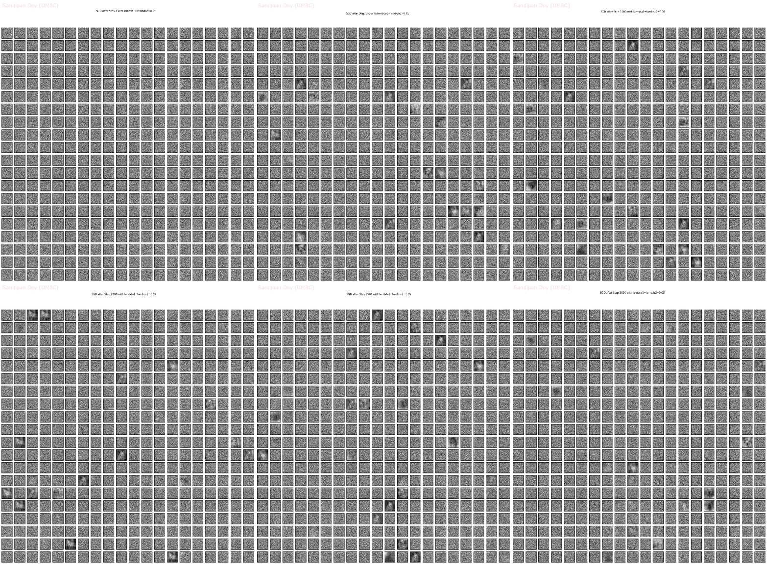
Clearly, the model learnt above overfits the training dataset, the test accuracy improved a bit, but still quite poor.

• Now, let’s train a deeper neural net with a two hidden layers, first one with 1024 nodes and second one with 64 nodes.
  
• Minibatch loss at step 0: 1015.947266
  Minibatch accuracy: 43.0%
  Validation accuracy: 50.0%
• Minibatch loss at step 500: 0.734610
  Minibatch accuracy: 79.7%
  Validation accuracy: 55.0%
• Minibatch loss at step 1000: 0.615992
  Minibatch accuracy: 93.8%
  Validation accuracy: 55.0%
• Minibatch loss at step 1500: 0.670009
  Minibatch accuracy: 82.8%
  Validation accuracy: 56.0%
• Minibatch loss at step 2000: 0.798796
  Minibatch accuracy: 77.3%
  Validation accuracy: 58.0%
• Minibatch loss at step 2500: 0.717479
  Minibatch accuracy: 84.4%
  Validation accuracy: 55.0%
• Minibatch loss at step 3000: 0.631013
  Minibatch accuracy: 90.6%
  Validation accuracy: 57.0%
• Minibatch loss at step 3500: 0.739071
  Minibatch accuracy: 75.8%
  Validation accuracy: 54.0%
• Minibatch loss at step 4000: 0.698650
  Minibatch accuracy: 84.4%
  Validation accuracy: 55.0%
• Minibatch loss at step 4500: 0.666173
  Minibatch accuracy: 85.2%
  Validation accuracy: 51.0%
• Minibatch loss at step 5000: 0.614820
  Minibatch accuracy: 92.2%
  Validation accuracy: 58.0%

Test accuracy: 55.2% 

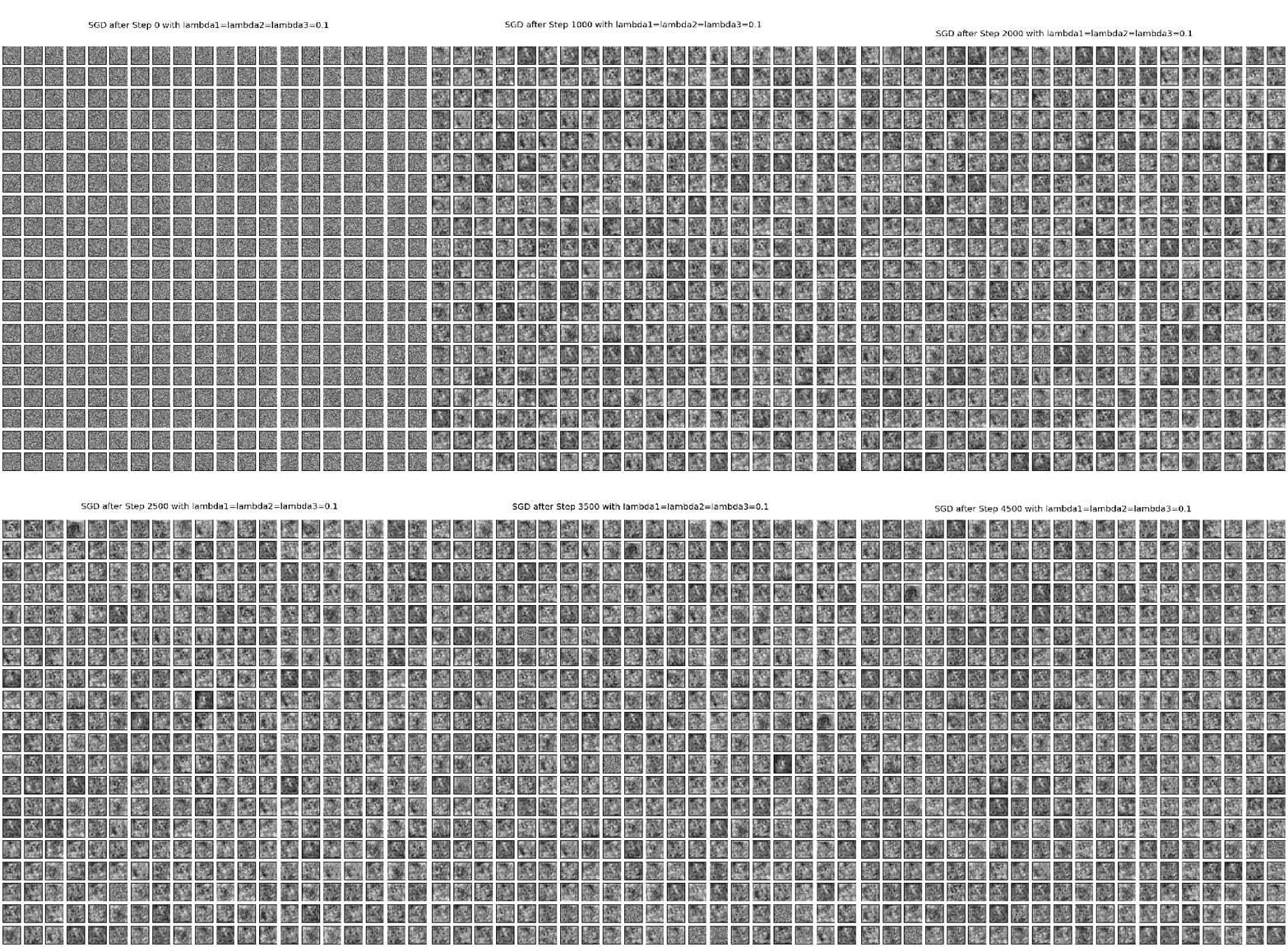
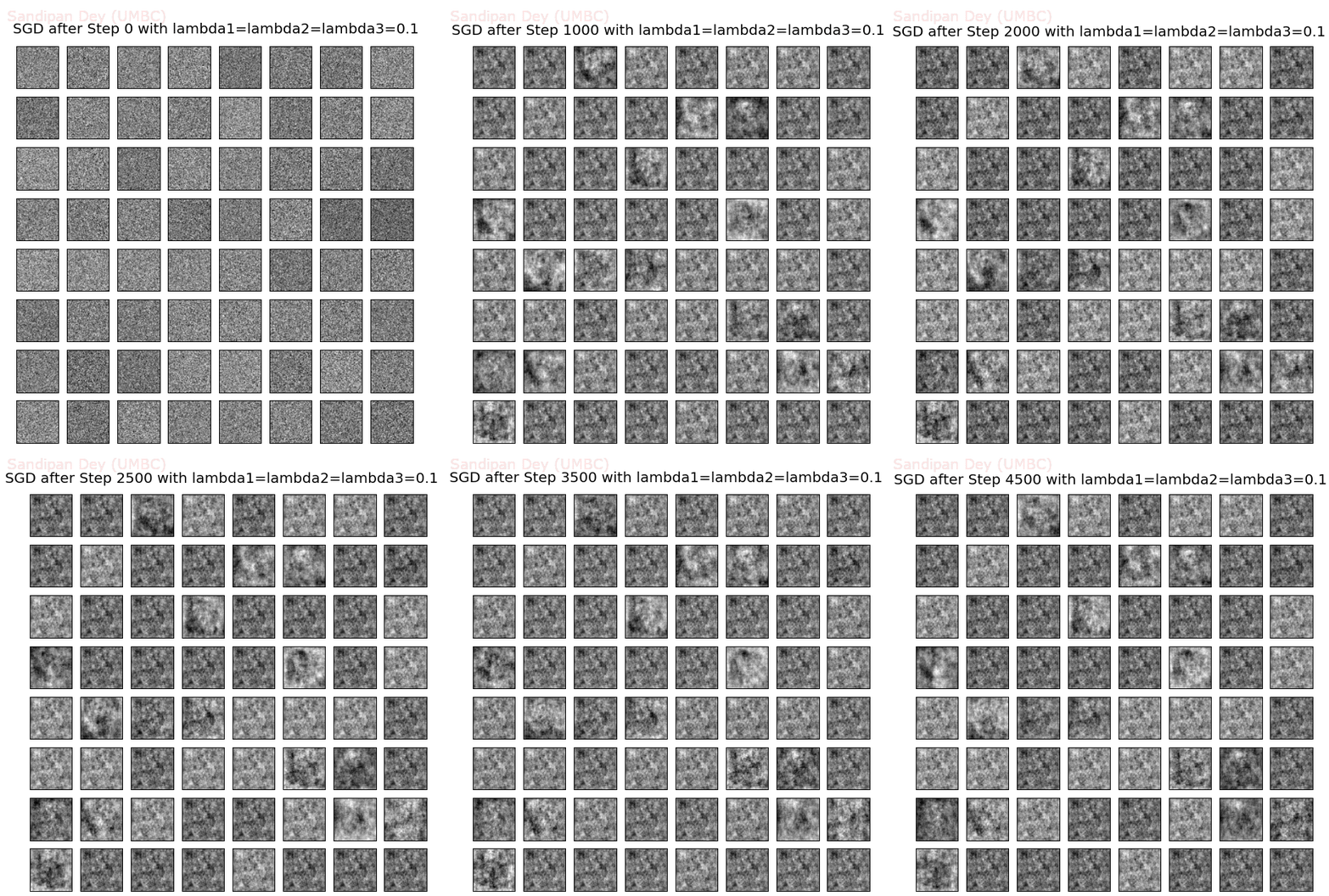
• The following animation visualizes the weights learnt for 400 randomly selected hidden units from the first hidden layer, by training the neural net model with SGD with L2-regularization (λ1=λ2=λ3=0.1, batch size=128, dropout rate=0.6). 

  

• The next animation visualizes the weights learnt and then the weights learnt for all the 64 hidden units for the second hidden layer.
• Clearly, the second deeper neural net model learnt above overfits the training dataset more, the test accuracy decreased a bit.

Classifying images with Deep Convolution Network

Let’s use the following conv-net shown in the next figure

As shown above, the ConvNet uses:

• 2 convolution layers each with
  • 5×5 kernel
  • 16 filters
  • 1×1 stride 
  • SAME padding
• 2 Max pooling layers each with
  • 2×2 kernel
  • 2×2 stride 
• 64 hidden nodes
• 128 batch size
• 5K iterations
• 0.7 dropout rate
• No learning decay
  

Results

Minibatch loss at step 0: 1.783917
Minibatch accuracy: 55.5%
Validation accuracy: 50.0%

Minibatch loss at step 500: 0.269719
Minibatch accuracy: 89.1%
Validation accuracy: 54.0%

Minibatch loss at step 1000: 0.045729
Minibatch accuracy: 96.9%
Validation accuracy: 61.0%

Minibatch loss at step 1500: 0.015794
Minibatch accuracy: 100.0%
Validation accuracy: 61.0%

Minibatch loss at step 2000: 0.028912
Minibatch accuracy: 98.4%
Validation accuracy: 64.0%

Minibatch loss at step 2500: 0.007787
Minibatch accuracy: 100.0%
Validation accuracy: 62.0%

Minibatch loss at step 3000: 0.001591
Minibatch accuracy: 100.0%
Validation accuracy: 63.0%

Test accuracy: 61.3% 

The following animations show the features learnt at different convolution and Maxpooling layers:

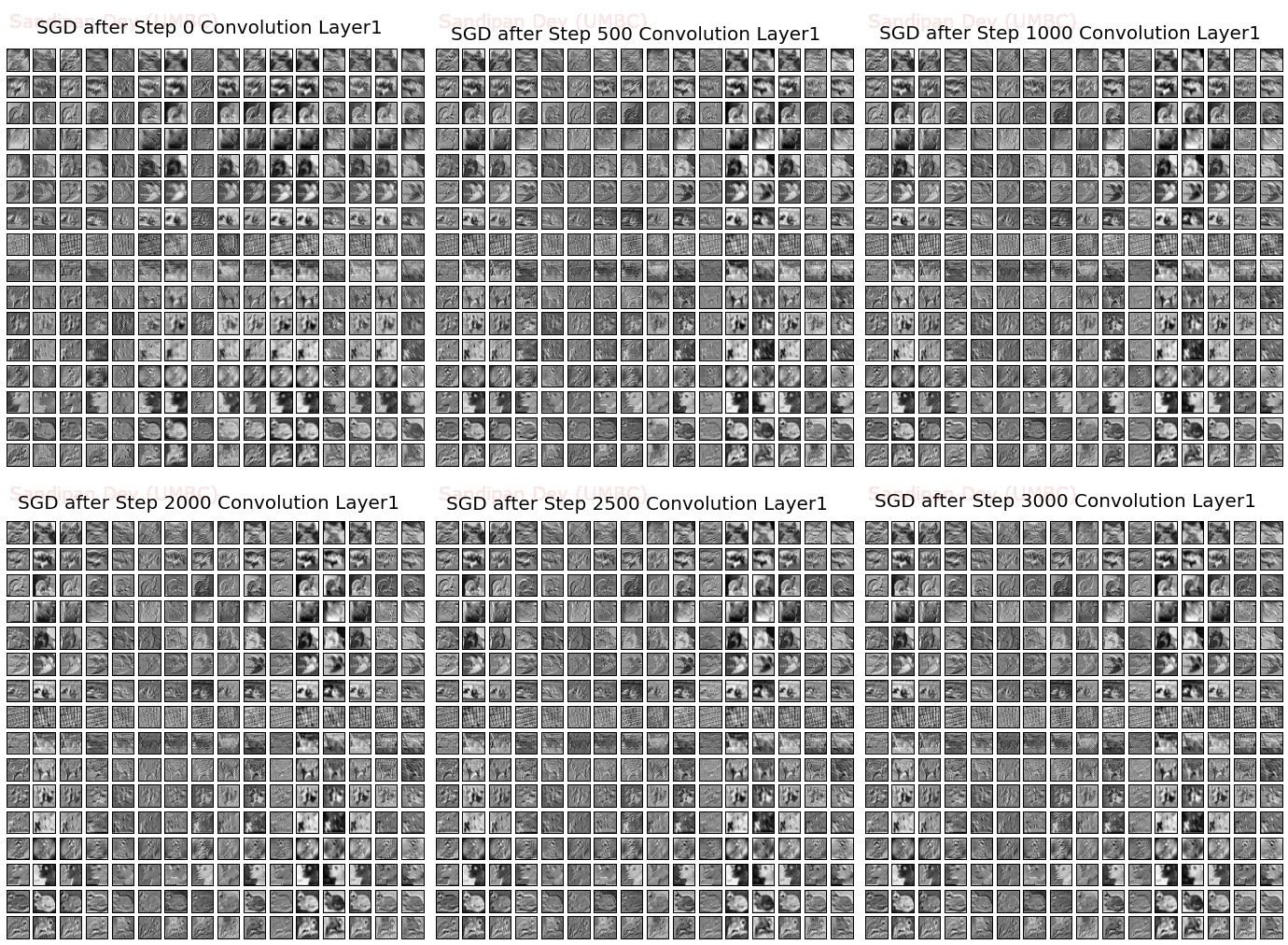
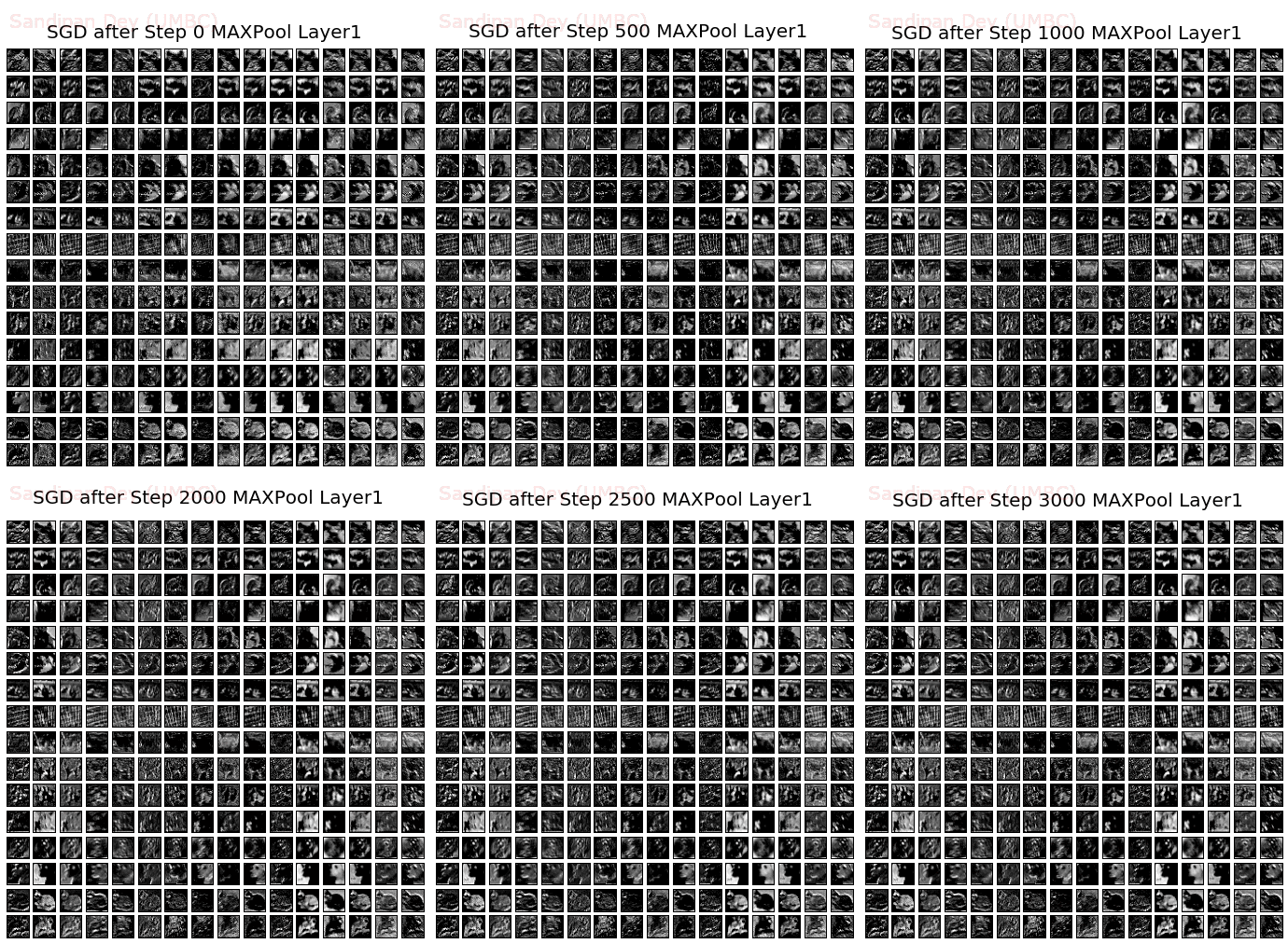
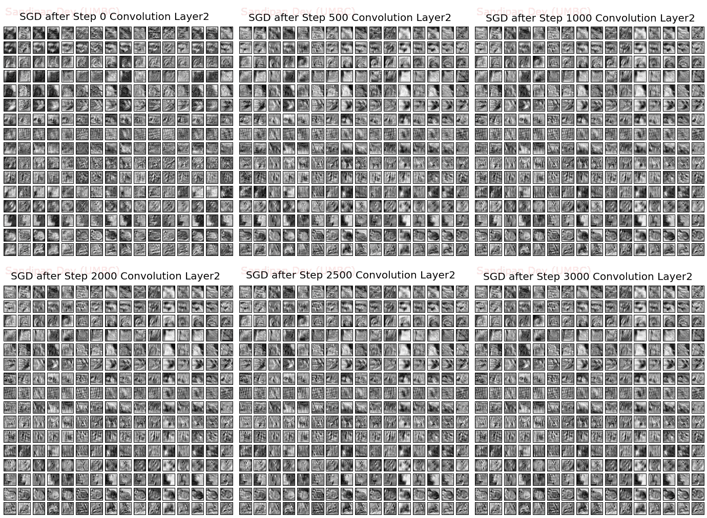
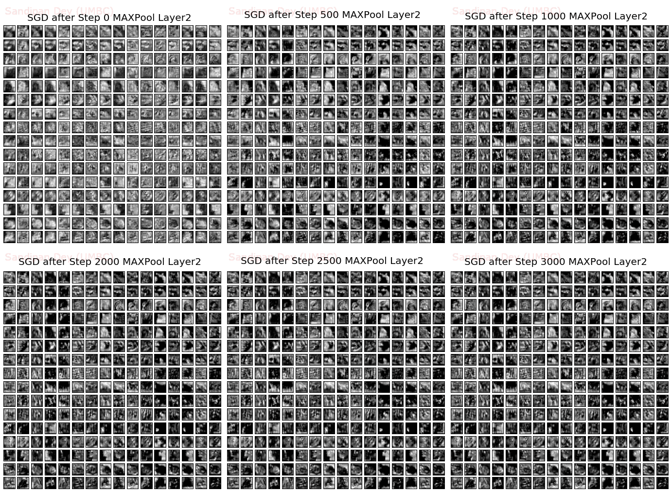
• Clearly, the simple convolution neural net outperforms all the previous models in terms of test accuracy, as shown below.

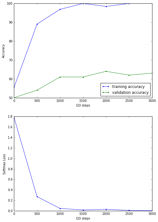
Only 1100 labeled images (randomly chosen from the training dataset) were used to train the model and predict 1000 test images (randomly chosen from the test dataset). Clearly the accuracy can be improved a lot if a large number of images are used fro training with deeper / more complex networks (with more parameters to learn).