Demystifying the Math of Support Vector Machines (SVM)

This article was written by Krishna Kumar Mahto.

So, three days into SVM, I was 40% frustrated, 30% restless, 20% irritated and 100% inefficient in terms of getting my work done. I was stuck with the Maths part of Support Vector Machine. I went through a number of YouTube videos, a number of documents, PPTs and PDFs of lecture notes, but everything seemed too indistinct for me. Out of all these, I found Andrew Ng’s Stanford lectures the most useful. Although he falls a little short in his ability to convey everything he intends to, his notes and derivations flow down very smoothly. Whatever I am going to discuss was inspired 50% by Andrew Ng’s lectures and his notes, 20% by one of the ML courses I am taking, and 29% by everything else and the rest of 1% comes from the little work which I put together into building this up. At the end, it turns out that it is not at all difficult to understand how SVM came up as all it takes is high school coordinate and vector geometry. For the most part, finding the right dots to make a sensible map was what I found difficult. With this article, I have tried to lay down the mathematical derivation which I came up with by affixing ideas from different sources, along with the thought process.

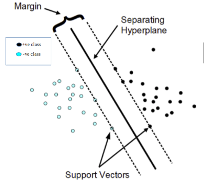
Fig 1. Diagrammatic representation of SVM for linearly separable dataset (Source: https://www.researchgate.net/figure/Classification-of-data-by-suppo…)

Let’s begin …

The diagram does not look to be too worrying if you know SVM at a high conceptual level (the Optimal Margin Classifier stuff). Although the cases of linearly separable datasets are not seen in real life, discussion throughout this article on SVM will be for this context only. I might do a separate post for a more general version of SVM.

SVM hypothesis: Hypothesis, w.r.t. a machine learning model is the model itself, which is nothing but our classifier (which, is a function).

Class labels: Class labels are denoted as -1 for negative class and +1 for positive class in SVM.

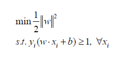
The final optimization problem that we shall have derived at the end of this article and what SVM solves to fit the best parameters is:

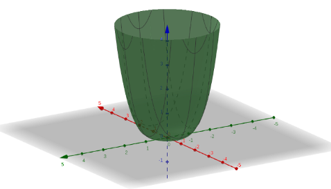
This is a convex optimization problem, with a convex optimization objective function and a set of constraints that define a convex set as the feasible region. Convex functions look like a bowl placed right-side-up. Convex set is a set of points in which a line joining any two points lies entirely within the set. I would have loved to talk on these in more detail, but it would be more convenient to just google the terms in italics.

Before delving into the actual part, we should be familiar with two terms- Functional margin and Geometric margin.

Functional margin and Geometric margin

Following is how we are going to notate the hyperplane that separates the positive and negative examples throughout this article:

Each training example is denoted as x, and superscript (i) denotes ith training example. In the following section y superscripted with (i) represents label corresponding to the ith training example.

Functional margin of a hyperplane w.r.t. ith taining example is defined as:

Functional margin of a hyperplane w.r.t. the entire dataset is defined as:

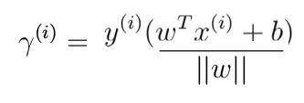
Geometric margin of a hyperplane w.r.t. ith training example is defined as functional margin normalized by norm(w):

Geometric margin for a hyperplane w.r.t. the entire dataset is defined as:

Note: In the following discussion, if it is not specified whether the functional/geometric margin of a hyperplane is mentioned w.r.t. the entire dataset or some example, then it should be assumed to be in reference to the entire dataset, and not a single example.

SVM maximizes the margin (as drawn in fig. 1) by learning a suitable decision boundary/decision surface/separating hyperplane. Second, SVM maximizes the geometric margin (as already defined, and shown below in figure 2) by learning a suitable decision boundary/decision surface/separating hyperplane. The way I have derived the optimization objective starts with using the concepts of functional and geometric margin; and after establishing that the two interpretations of SVM coexist with each other, the final optimization objective is derived.

To read the whole article, with illustrations and formulas, click here.

DSC Resources