The following problems appeared in the first few assignments in the Udacity course Deep Learning (by Google). The descriptions of the problems are taken from the assignments.
Classifying the letters with notMNIST dataset
Let’s first learn about simple data curation practices, and familiarize ourselves with some of the data that are going to be used for deep learning using tensorflow. The notMNIST dataset to be used with python experiments. This dataset is designed to look like the classic MNIST dataset, while looking a little more like real data: it’s a harder task, and the data is a lot less ‘clean’ than MNIST.
Preprocessing
First the dataset needs to be downloaded and extracted to a local machine. The data consists of characters rendered in a variety of fonts on a 28×28 image. The labels are limited to ‘A’ through ‘J’ (10 classes). The training set has about 500k and the testset 19000 labelled examples. Given these sizes, it should be possible to train models quickly on any machine.
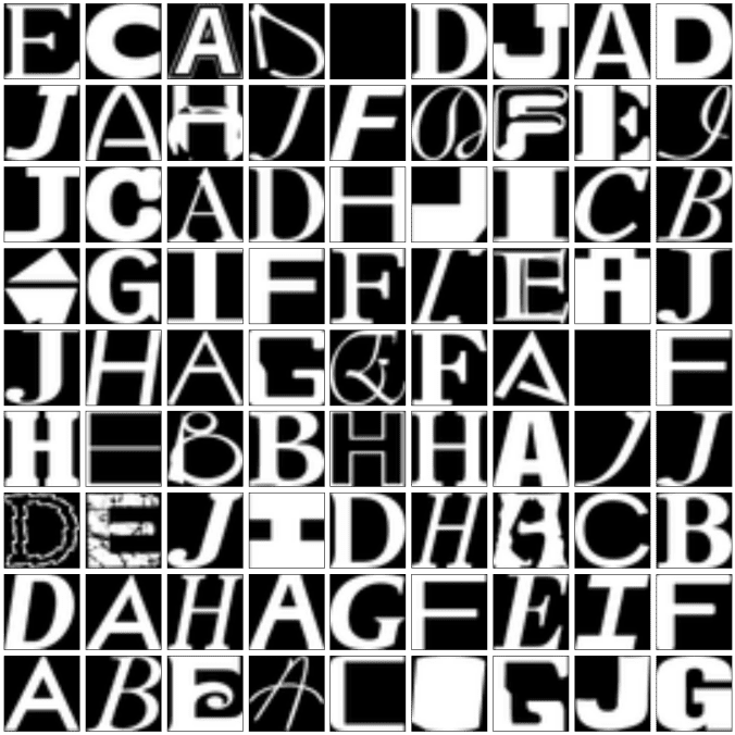
Let’s take a peek at some of the data to make sure it looks sensible. Each exemplar should be an image of a character A through J rendered in a different font. Display a sample of the images downloaded.
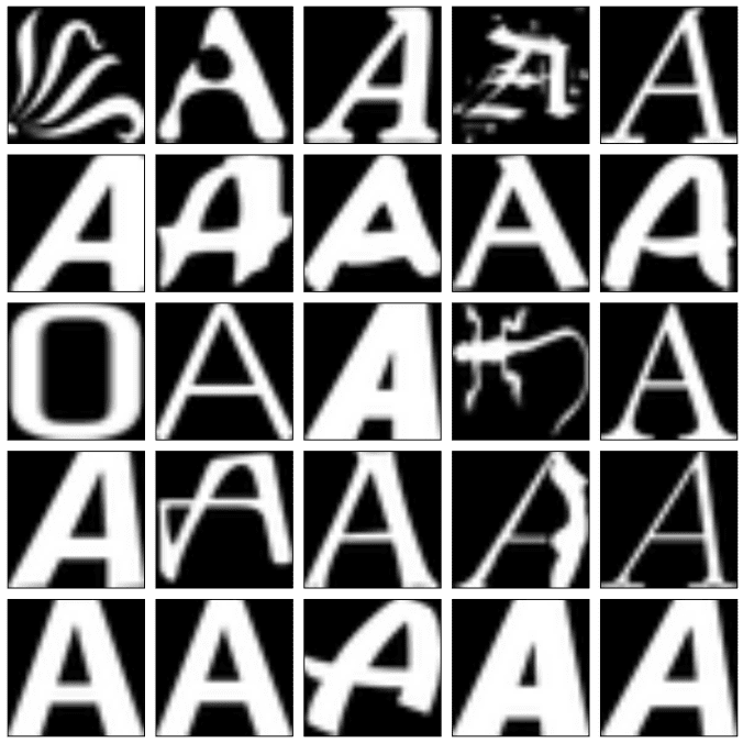
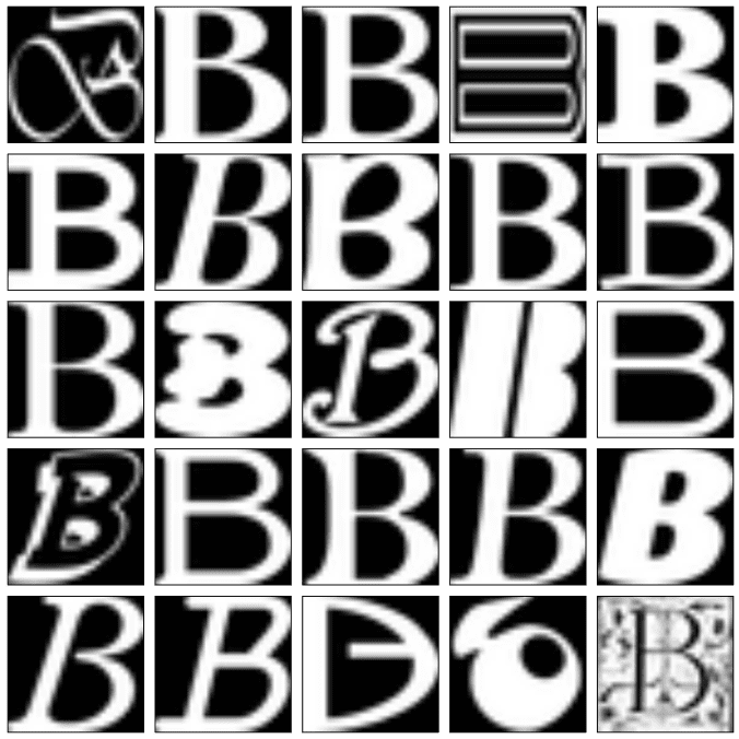
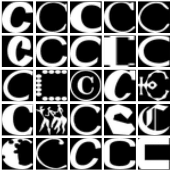
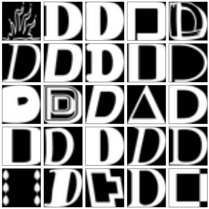
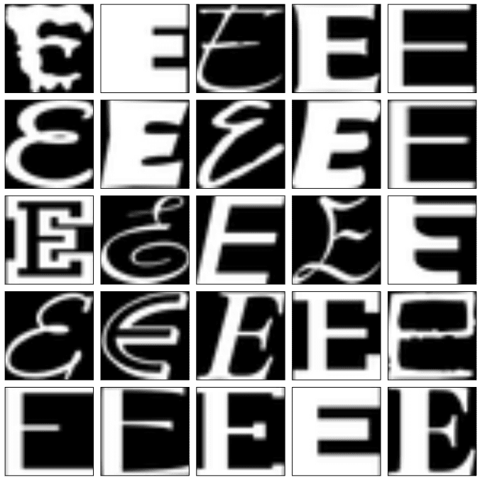
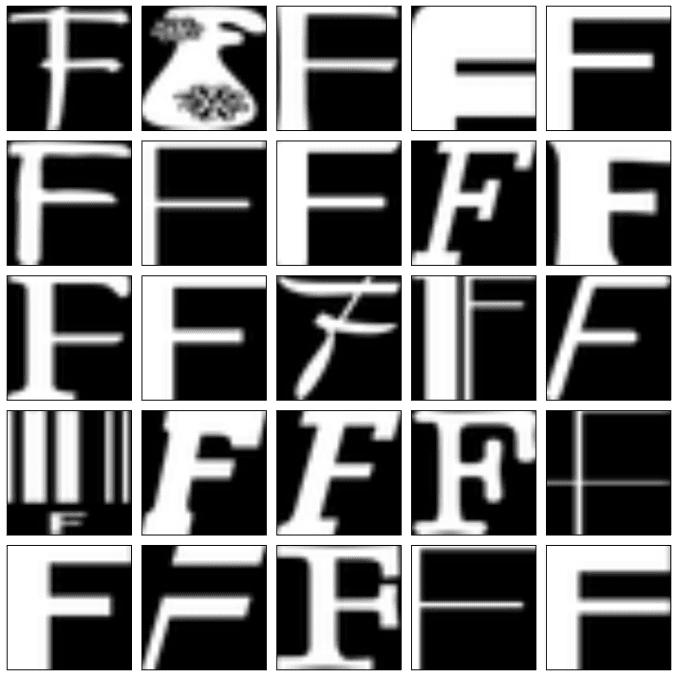
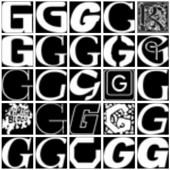
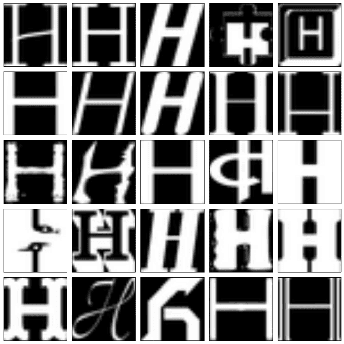
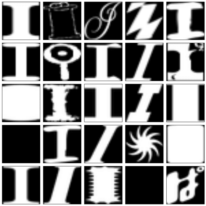
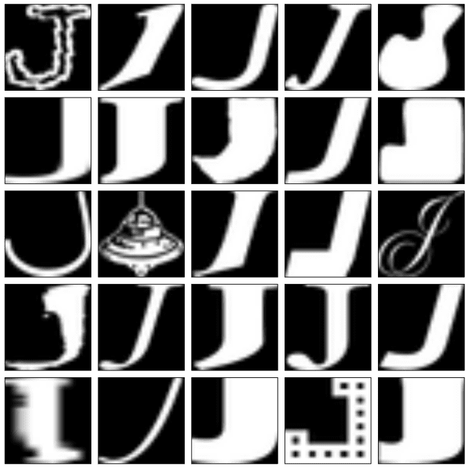
Now let’s load the data in a more manageable format. Let’s convert the entire dataset into a 3D array (image index, x, y) of floating point values, normalized to have approximately zero mean and standard deviation ~0.5 to make training easier down the road. A few images might not be readable, we’ll just skip them. Also the data is expected to be balanced across classes. Let’s verify that. The following output shows the dimension of the ndarray for each class.
Now some more preprocessing is needed:
- First the training data (for different classes) needs to be merged and pruned.
- The labels will be stored into a separate array of integers from 0 to 9.
- Also let’s create a validation dataset for hyperparameter tuning.
- Finally the data needs to be randomized. It’s important to have the labels well shuffled for the training and test distributions to match.
After preprocessing, let’s peek a few samples from the training dataset and the next figure shows how it looks.
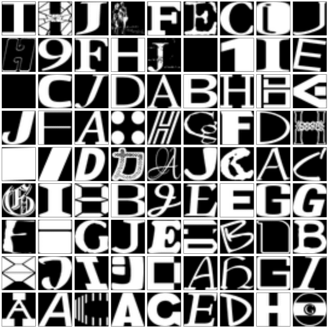
Here is how the validation dataset looks (a few samples chosen).
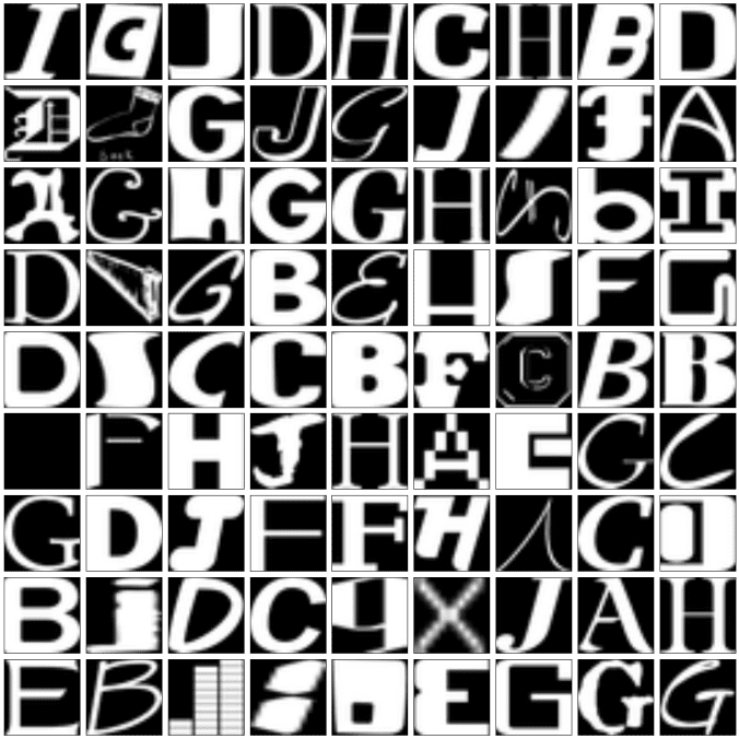
Here is how the test dataset looks (a few samples chosen).
Trying a few off-the-self classifiers
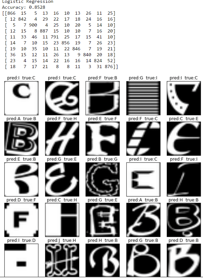
Let’s get an idea of what an off-the-shelf classifier can give us on this data. It’s always good to check that there is something to learn, and that it’s a problem that is not so trivial that a canned solution solves it. Let’s first train a simple LogisticRegression model from sklearn (using default parameters) on this data using 5000 training samples.
The following figure shows the output from the logistic regression model trained, its accuracy on the test dataset (also the confusion matrix) and a few test instances classified wrongly (predicted labels along with the true labels) by the model.
Deep Learning with TensorFlow
Now let’s progressively train deeper and more accurate models using TensorFlow. Again, we need to do the following preprocessing:
- Reformat into a shape that’s more adapted to the models we’re going to train: data as a flat matrix,
- labels as 1-hot encodings.
Now let’s train a multinomial logistic regression using simple stochastic gradient descent.
TensorFlow works like this:
First we need to describe the computation that is to be performed: what the inputs, the variables, and the operations look like. These get created as nodes over a computation graph.
Then we can run the operations on this graph as many times as we want by calling session.run(), providing it outputs to fetch from the graph that get returned.
- Let’s load all the data into TensorFlow and build the computation graph corresponding to our training.
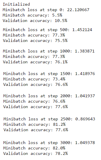
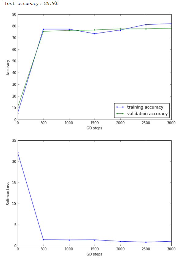
- Let’s use stochastic gradient descent training (with ~3k steps), which is much faster. The graph will be similar to batch gradient descent, except that instead of holding all the training data into a constant node, we create a Placeholder node which will be fed actual data at every call of session.run().
Logistic Regression with SGD
The following shows the fully connected computation graph and the results obtained.

Neural Network with SGD
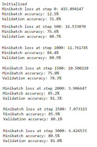
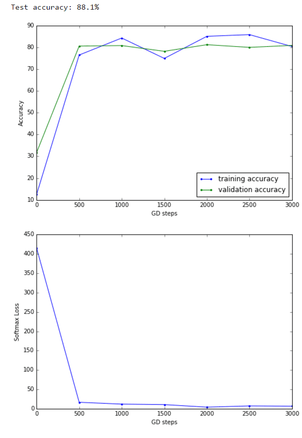
Now let’s turn the logistic regression example with SGD into a 1-hidden layer neural network with rectified linear units nn.relu() and 1024 hidden nodes. As can be seen from the below results, this model improves the validation / test accuracy.
Regularization with Tensorflow
Previously we trained a logistic regression and a neural network model with Tensorflow. Let’s now explore the regularization techniques.
Let’s introduce and tune L2regularization for both logistic and neural network models. L2 amounts to adding a penalty on the norm of the weights to the loss. In TensorFlow, we can compute the L2loss for a tensor t using nn.l2_loss(t).
The right amount of regularization improves the validation / test accuracy, as can be seen from the following results.
L2 Regularized Logistic Regression with SGD
The following figure recapitulates the simple network without anyt hidden layer, with softmax outputs.

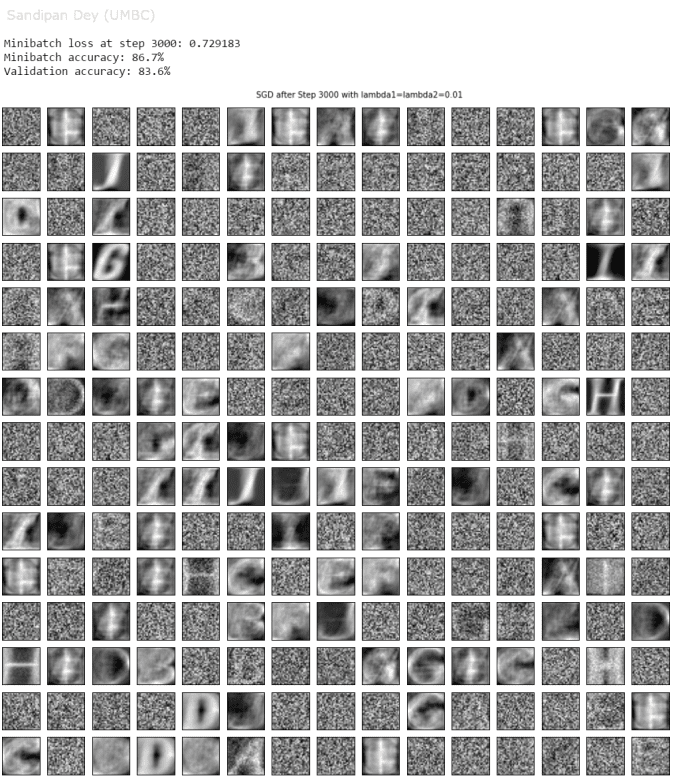
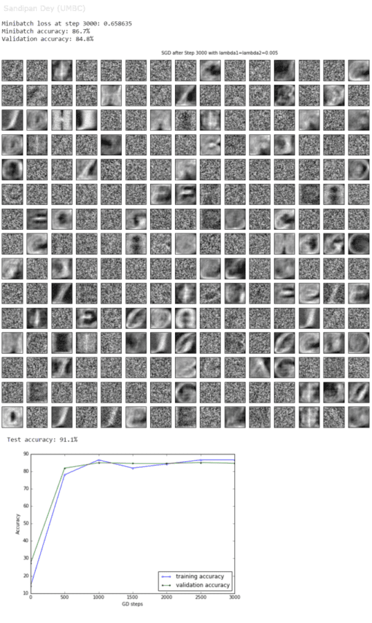
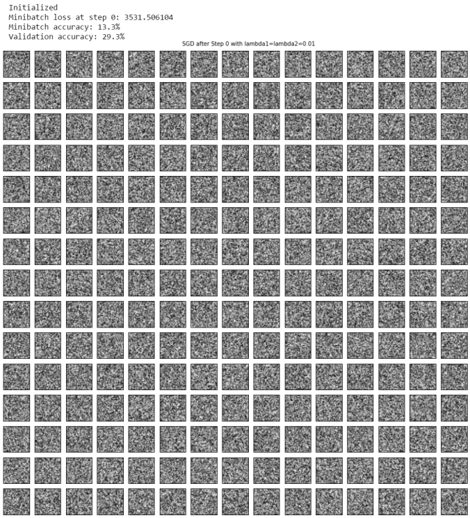
The next figures visualize the weights learnt for the 10 output neurons at different steps using SGD and L2 regularized loss function (with λ=0.005). As can be seen below, the weights learnt are gradually capturing the different features of the letters at the corresponding output neurons.
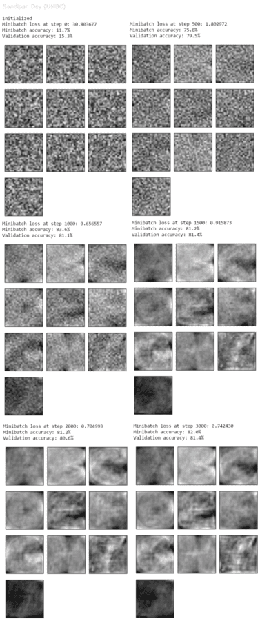
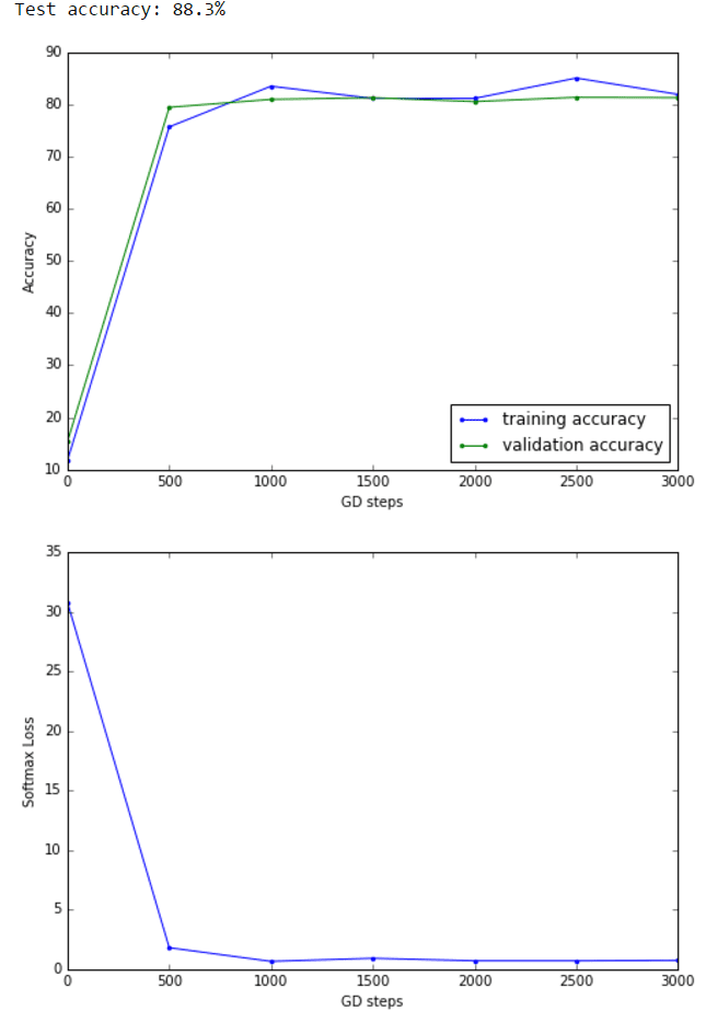
As can be seen, the test accuracy also gets improved to 88.3% with L2 regularized loss function (with λ=0.005).
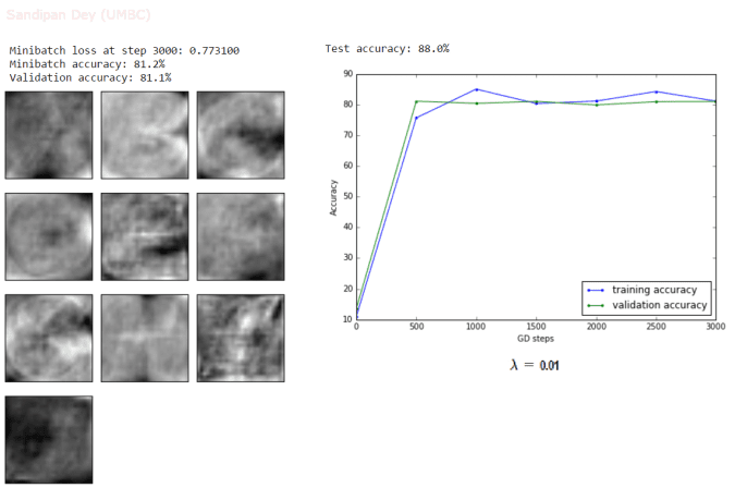
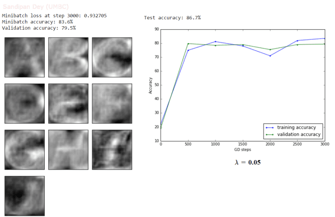
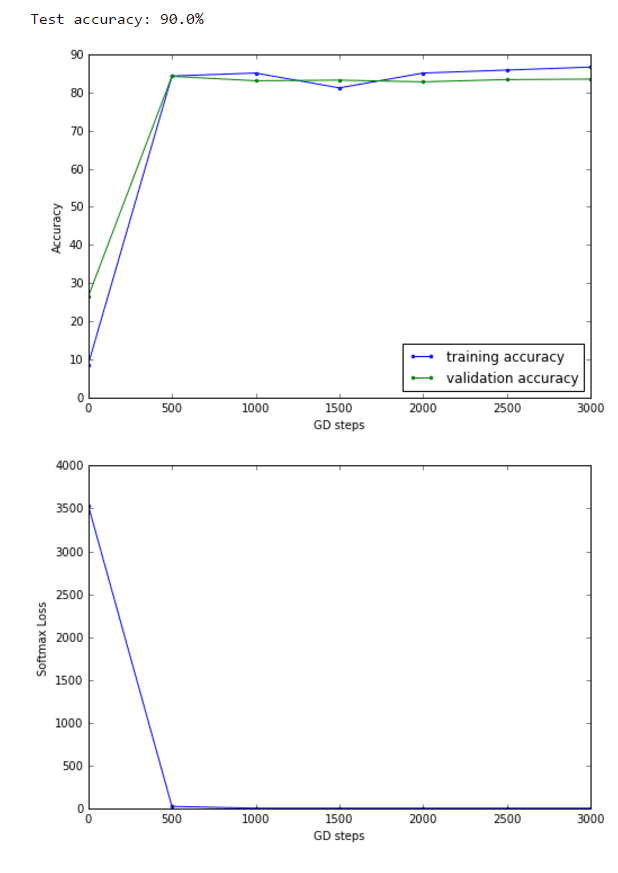
The following results show the accuracy and the weights learnt for couple of different values of λ (0.01 and 0.05 respectively). As can be seen, with higher values of λ, the logistic regression model tends to underfit and test accuracy decreases.
L2 Regularized Neural Network with SGD
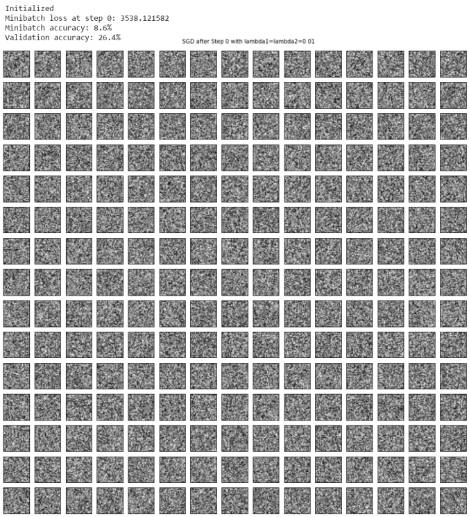
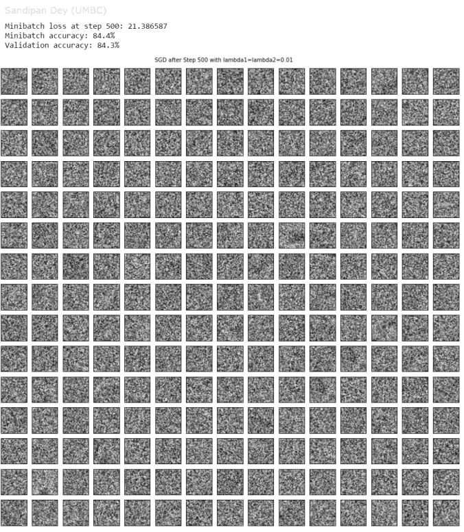
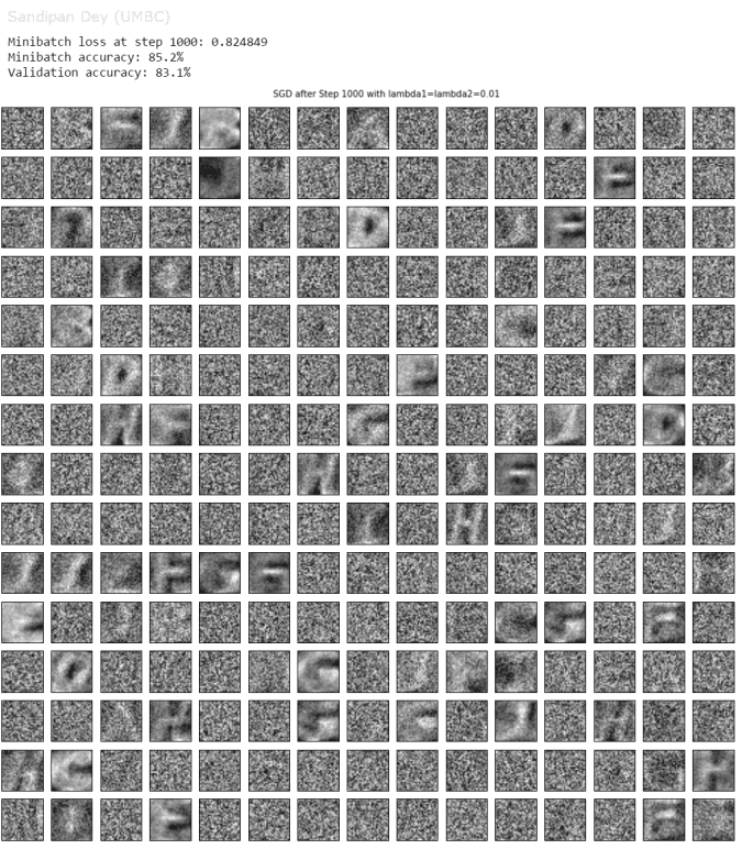
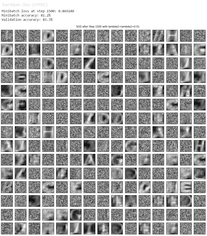
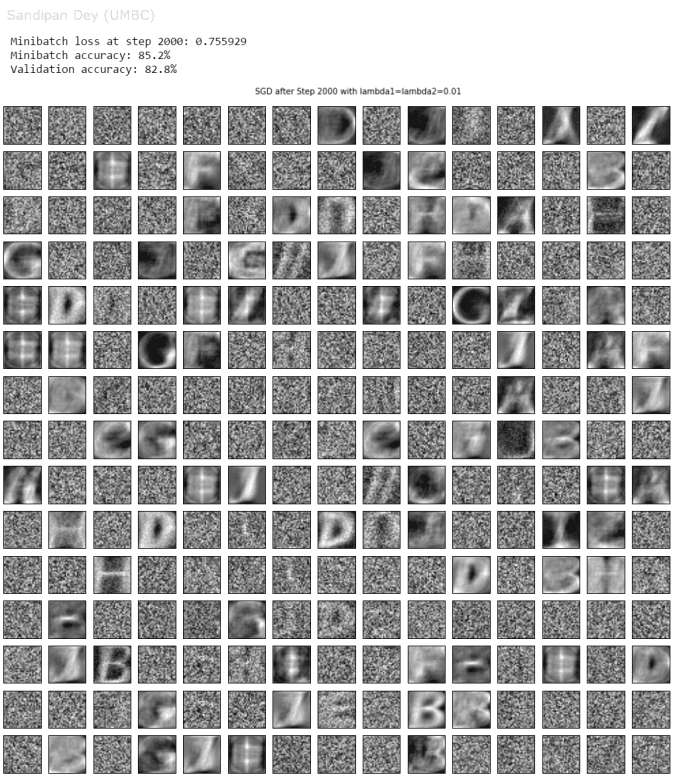
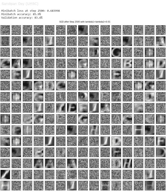
The following figure recapitulates the neural network with a single hidden layer with 1024 nodes, with relu intermediate outputs. The L2 regularizations applied on the loss function for the weights learnt at the input and the hidden layers are λ1 and λ2, respectively.

Overfitting
Let’s demonstrate an extreme case of overfitting. Restrict your training data to just a few batches. What happens?
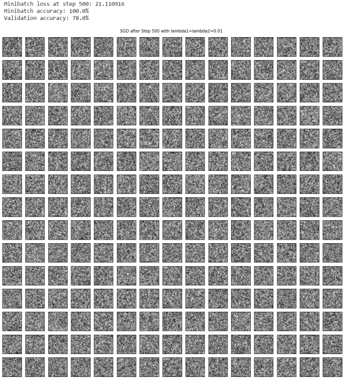
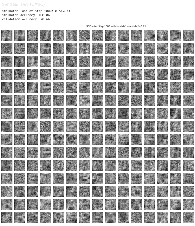
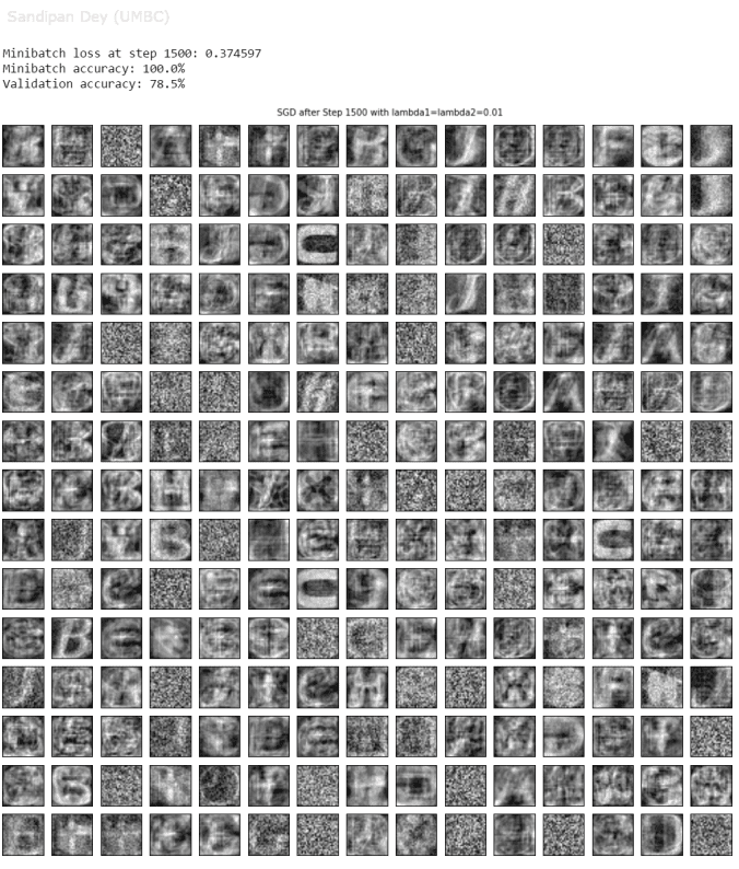
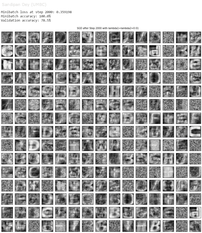
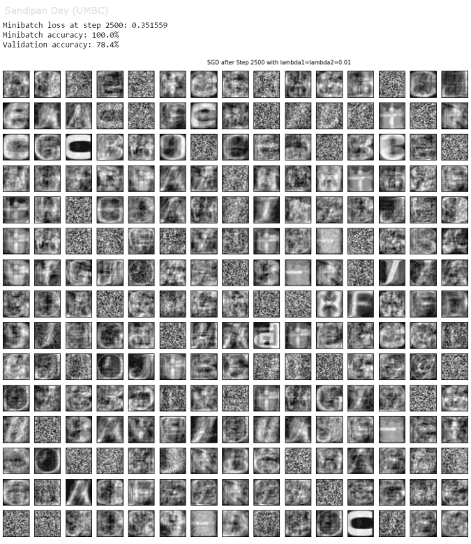
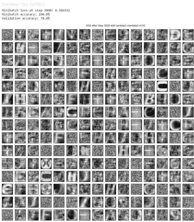
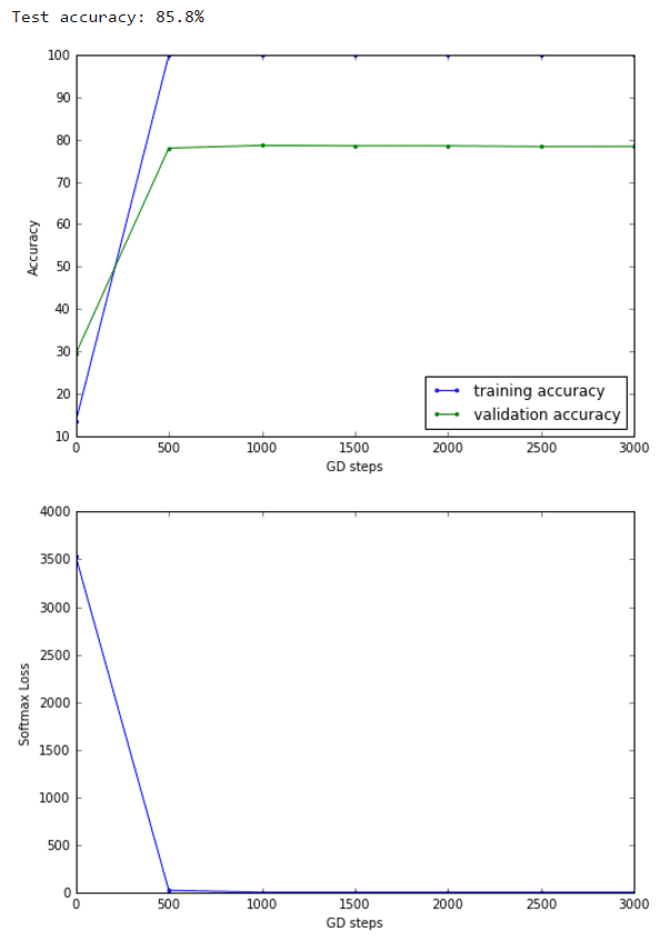
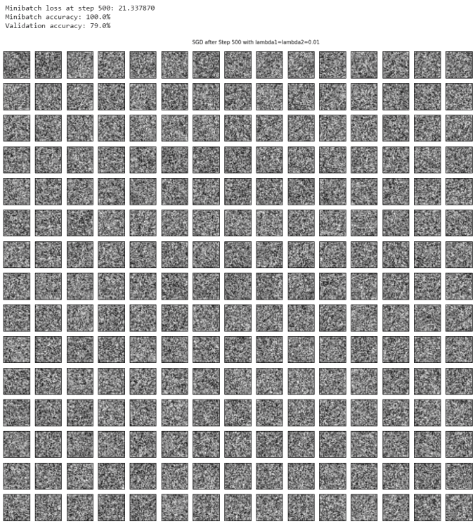
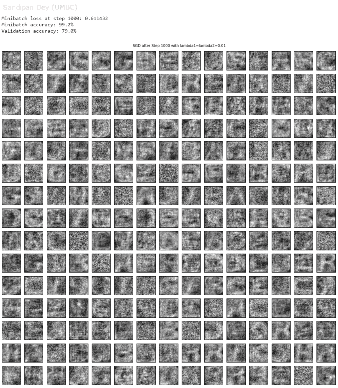
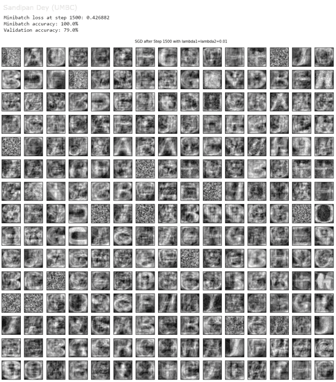
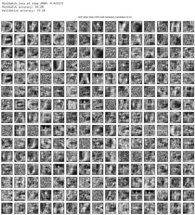
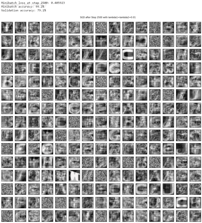
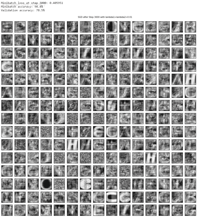
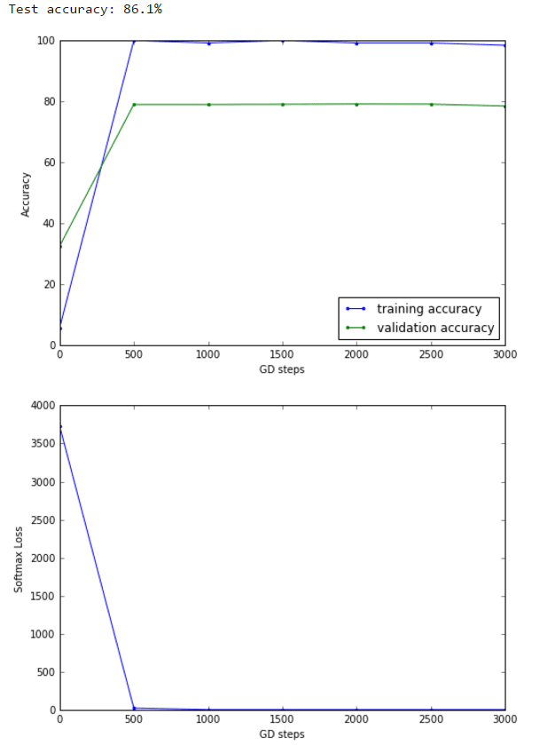
Let’s restrict the training data to n=5 batches. The following figures show how it increases the training accuracy to 100% (along with a visualization of a few randomly-picked input weights learnt) and decreases the validation and the test accuracy, since the model is not generalized enough.
Dropouts
Introduce Dropout on the hidden layer of the neural network. Remember: Dropout should only be introduced during training, not evaluation, otherwise our evaluation results would be stochastic as well. TensorFlow provides nn.dropout() for that, but you have to make sure it’s only inserted during training.
What happens to our extreme overfitting case?
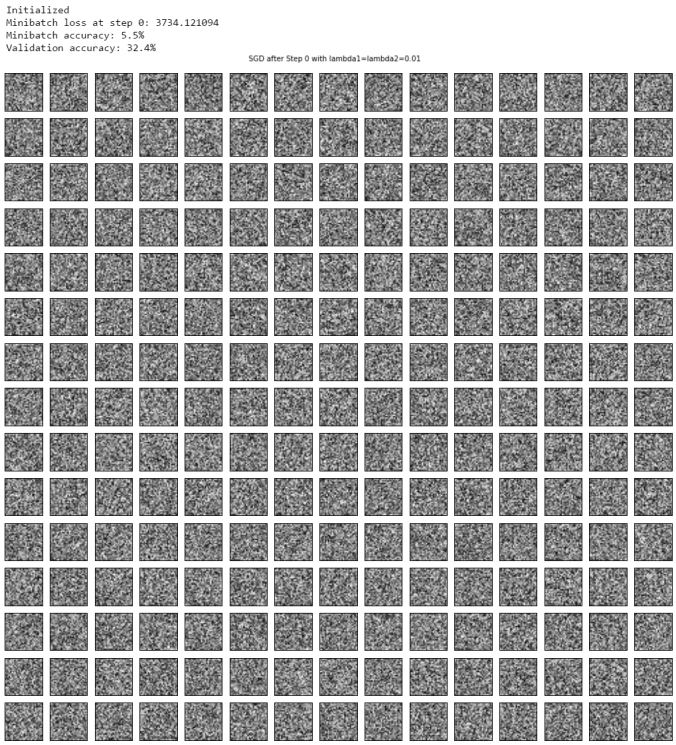
As we can see from the below results, introducing a dropout rate of 0.4 increases the validation and test accuracy by reducing the overfitting.
Till this point the highest accuracy on the test dataset using a single hidden-layer neural network is 91.1%. More hidden layers can be used / some other techniques (e.g., exponential decay in learning rate can be used) to improve the accuracy obtained (to be continued…).
