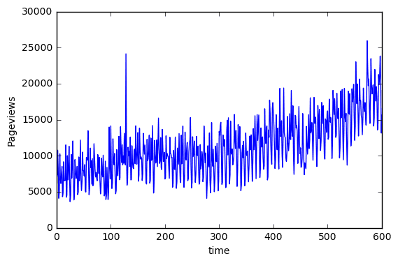
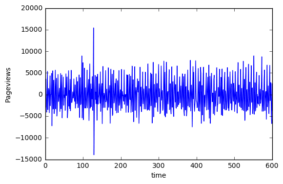
The trend and seasonality can be accounted for in a linear model by including sinusoidal components with a given frequency. However, finding the appropriate frequency for each sinusoidal component requires a little more digging. This post shows how to use fast Fourier transforms to find these frequencies.
Defining the model:
y = P(t) + S(t) + T(t) + R(t)
- P(t)~Polynomial component
- S(t)~Seasonal component
- T(t)~Trend component
- R(t)~Residual error
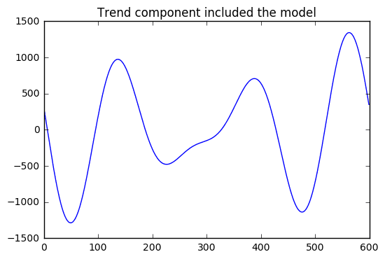
For the purposes of this post, we will only focus on the T(t) and S(t) components. The actual model fitting will be done in a separate post.
600 observations were used in the training set. The result was tested on the full dataset with 731 observations.
Find the overall trend:
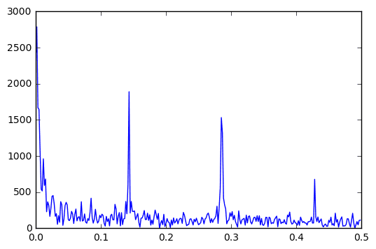
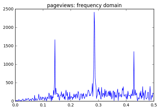
I used an FFT transformation to visualize the magnitude of the frequency components in the time series. To be specific, the absolute magnitude is plotted.
Frequency Component, Magnitude
[  1.41666667e-01   1.82239797e+05]
[  1.43333333e-01   5.67160341e+05]
 [  2.83333333e-01   1.66899918e+05]
 [  2.85000000e-01   4.59942544e+05]
 [  2.86666667e-01   3.95441559e+05]
 [  4.28333333e-01   2.03492985e+05]
Does it make sense to reuse frequencies for the trend and seasonal components?
- On one hand, it might be better not to miss anything. I doubt there will be a prominant trend for -a weekday- every 28 weeks.
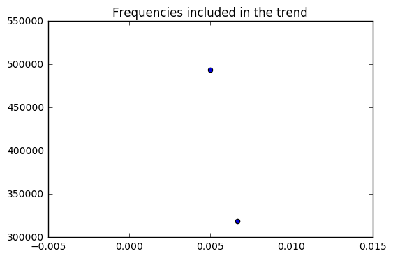
- For the trend component, it would makes sense to use the lowest frequencies with the highest magnitudes.
- For the seasonal component, there are “interesting” frequencies around .143, .285, and .428.
Finding seasonal patterns in the target variable:
The overall trend could be removed by creating a differenced variable for Pageviews The differenced variable allows for seasonal components to be identified more clearly.
The lower frequency components were removed and the other, distinct frequencies were amplified. This makes the frequencies easier to filter! Also it makes it easier to compare to possible seasonal variables.
Finding the seasonal predictor variable:
Frequency Component, Magnitude
[  1.41666667e-01   2.42782136e+02]
[  1.43333333e-01   6.00386477e+02]
 [  1.45000000e-01   1.31981640e+02]
 [  2.85000000e-01   2.78344410e+02]
 [  2.86666667e-01   2.07887576e+02]
 [  4.28333333e-01   2.97539156e+02]
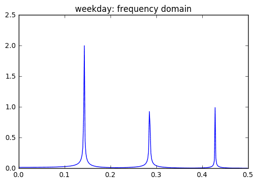
Eureka! Weekday shares the same frequency components as Pageviews!
I found dominant frequencies at .143, .285, and .428. These correspond to T=7.14,3.5, and 2.33. There were also some frequencies around the e-3 orders of magnitude. These were at .00166, .00333, and 0.005 and had periods upwards of 200.
If you want to see how I included these frequency components in a regression model please see my Github. The results are compared to straight up dummy coding (the results are the same).

