Bernoulli Lattice Models - Connection to Poisson Processes

Bernouilli lattice processes may be one of the simplest examples of point processes, and can be used as an introduction to learn about more complex spatial processes that rely on advanced measure theory for their definition. In this article, we show the differences and analogies between Bernouilli lattice processes on the standard rectangular or hexagonal grid, and the Poisson process, including convergence of discrete lattice processes to continuous Poisson process, mainly in two dimensions. We also illustrate that even though these lattice processes are purely random, they don’t look random when seen with the naked eye.

We discuss basic properties such as the distribution of the number of points in any given area, or the distribution of the distance to the nearest neighbor. Bernouilli lattice processes have been used as models in financial problems, see here. Most of the papers on this topic are hard to read, but here we discuss the concepts in simple English. Interesting number theory problems about sums of squares, deeply related to these lattice processes, are also discussed. Finally, we show how to identify if a particular realization is from a Bernouilli lattice process, a Poisson process, or a combination of both.

See below a realization of a Bernouilli process on the regular hexagonal lattice. The main feature of such a process is that the point locations are fixed, not random. But whether a point is “fired” or not (that is, marked in blue) is purely random and independent of whether any other point is fired or not. The probability for a point to be fired is a Bernouilly variable of parameter p.

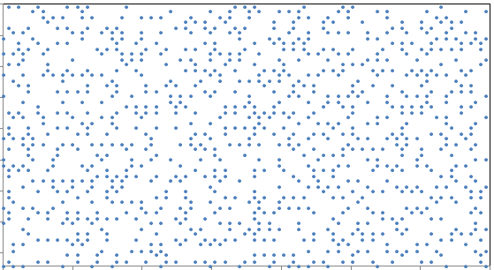
Figure 1: realization of Bernouilli hexagonal lattice process

The source code to produce this plot is available here. More sophisticated models, known as Markov random fields, allows for neighboring points to be correlated. They are useful in image analysis, see here and here.

To the contrary, Poisson processes assume that the point locations are random. The points being fired are uniformly distributed on the plane, and not restricted to integer or grid coordinates. In short, Bernouilli lattice processes are discrete approximations to Poisson processes. Below is an example of a realization of a Poisson process.

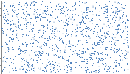
Figure 2: realization of a Poisson process

1. Definition and Convergence to Poisson Process

We are dealing here with square lattices covering the entire two-dimensional plane. A point of the lattice is a vector (rx, ry) where x, y are integers (positive or negative) and r a strictly positive real number, called the scale of the lattice. A Bernouilli variable is attached to each point: it is equal to 1 with probability p, and to 0 with probability 1 – p. A point of the lattice is said to be fired if its Bernouilli variable is equal to 1. Such points are marked in blue in all the plots. The Bernouilli variables are independent and have the same parameter p: in other words, this 2-parameter lattice process is homogeneous, as p does not depend on the location.

We compare these processes to homogeneous Poisson process of intensity λ, covering the entire plane. For Poisson processes, point locations are random, see figure 2. The number of points in any given area D has a Poisson distribution with mean λ S(D), where S represents the surface of the area. The distance to the nearest neighbor has the following distribution, see here:

1.1. Poisson approximation to Bernouilli lattice process

In the same way that Bernouilli variables are approximated by Poisson variables when p is small, Bernouilli processes are approximated by Poisson processes when p is small. The parameters p and λ play the same role.

The way convergence occurs is very intuitive. Start with a Bernouilli lattice process as pictured in figure 3, with r = 1. Reduce r by a factor 2 and p by a factor 4: see result in figure 4. Keep repeating this step indefinitely, and you end up with figure 2.

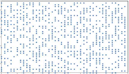
Figure 3: Realization of a Bernouilli square lattice process

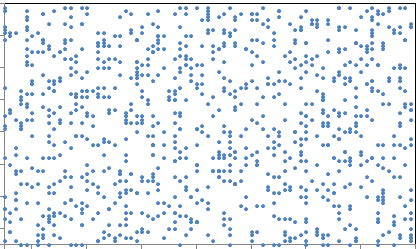
Figure 4: A more granular version, with smaller r and p

2. Properties of Bernouilli lattice processes

As for Poisson processes, two main features are:

the distribution between a point of the lattice and its closest “blue” neighbor
the distribution of the number of blue points in any given area.

The number N of blue points in any given area D is a Binomial variable with expectation p S(D), with S(D) being the total number of lattice points (blue or not) in D. That is,

For any lattice point z, let Y be the distance to the closest blue neighbor. Let D be a circle centered at z, with radius y. The probability that Y is larger than y is the probability that there is no blue point in D, that is, based on the previous formula:

Note that if z is a blue point, it is not considered to be a nearest neighbor to itself.

2.1. More about the Poisson approximation

When r and p get smaller and smaller as discussed in section 1.1, we have convergence to the Poisson process, and S(D) in the above formula (for Bernouilli lattice processes) tends to the surface area of D, that is

Likewise, for the Poisson process, based on the first formula in section 1, when λ is small, we have

Now the analogy with Poisson processes becomes more clear. Also, p and λ are equivalent, at the limit. Below is the distribution of Y for a Bernouilli lattice process with p = 0.001.

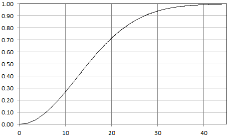
Figure 5: Distribution of distance to nearest neighbor: P(Y < y)

It is indistinguishable from that of a Poisson process with λ = 0.001. There is a major difference though: the distribution is a discrete one for the lattice process, and a continuous one for the Poisson process, but you can’t tell the difference with the naked eye, for such a small value of p.

2.2. Model testing

Since Poisson and Bernouilli lattice processes can be quite similar depending on the granularity of the lattice, one might be interested in testing if some observed data fits with either model. An easy test involves computing the empirical distribution of the distance to the nearest neighbor, and check whether it fits the Bernouilli lattice or Poisson theoretical distribution.

For blended models, say a mixture of Poisson and Bernouilli lattice, one can do simulations. Simulations will also allow you to estimate the proportions of Bernouilli versus Poisson in the mixture model.

2.3. Connection to number theory: sums of two squares

An interesting result that can easily be derived from the formulas in section 2.1 is the following. The number of (x, y) solution to x^2 + y^2 ≤ n, where n is a positive integer and the unknown x, y are positive or negative integers, tends to π n as n tends to infinity. This is known as the Gauss circle problem. So, on average, the equation x^2 + y^2 = n has π solutions, though for some n, for instance n = 1105, it can be much higher (32 in this case). Source code to compute the number of solutions is available here. More generally, the number of integer solutions to such inequalities can be approximated by the surface area under the curve using integration techniques, the curve here being x^2 + y^2 ≤ n.

A deeper result is the following. Let r(n) be the number of solutions to x^2 + y^2 = n. This function is known as the sum of squares function. For k between n and 2n, we have

integers such that r(k) > 0, based on this well known result, where c = 0.7642… is the Landau-Ramanujan constant. Also, based on the Gauss circle problem, the total number of solutions across all k‘s between n and 2n is asymptotically 2π n − π n = π n. These π n solutions are distributed across cn / SQRT(log n) integers satisfying r(k) > 0. This means that for large n‘s satisfying r(n) > 0, the average value of r(n) grows as π SQRT(log n) / c. A consequence of this is that the records for r(n) grow faster than π SQRT(log n) / c. How much faster?

Technical note: Sums of squares are far more abundant than primes, yet their natural density is also zero. This means that as n becomes larger and larger, the chance for n to be a sum of two squares, tends to zero. But for the few remaining n‘s that can be expressed as a sum of two squares, the number of ways they can be expressed that way, increases more and more on average. That is, r(n) tends to increase with n, for those few large n satisfying r(n) > 0. As a result, for any n large or small, the number of solutions to x^2 + y^2 = n is equal to π on average. What changes (it increases) when n is large is the probability that r(n) = 0, but the average value of r(n) remains unchanged.

More about sums of squares in the context of number theory, can be found here and here. See also this post and this article.

3. Related articles by same author

Here is a selection of articles pertaining to experimental math and probabilistic number theory:

Bernoulli Lattice Models – Connection to Poisson Processes

Leave a Reply Cancel reply