Recommender systems are applied in a variety of industries such as e-commerce, streaming services and others. There are two major techniques used in Recommender systems, collaborative filtering and Content-based filtering. This article presents five “Jupyter” NoteBooks which construct a large scale recommender system based on a collaborative filter using Spark FrameWork SVD, and another using Amazon Sage Maker AutoEncode. The dataset used has more than 28 million user ratings. In this article the final results of the two techniques are shown and compared and Spark SVD brings better results.
There are two major techniques used in Recommender systems: collaborative filtering with recommend items based on the users’ previous actions. Content-based filtering approaches utilize the characteristics of items in order to recommend additional items with similar properties. it’s possible to use one of these techniques, however, a hybrid solution is also possible which combines both.
The most common collaborative filtering techniques involve the use of a correlation matrix which is based on the user’s actions, associating each user with each item in your model. The big problem for this kind of solution is scalability. In systems with millions of users and items you produce matrixes with trillions of cells which are not easy to work with. To overcome this kind of problem there are techniques to reduce the dimensions of the matrix and also Spark, a framework for large datasets.
Normally, before applying a suggestion algorithm you have to acquire and prepare the dataset. The dataset used was acquired by searching through many library sites and social network pages, collecting the user ratings of books. The first notebook SparJoinTable.ipynb prepared the acquired datasets to be used in the social filtering algorithms.
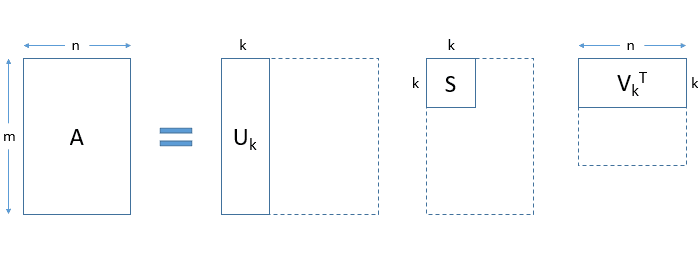
The dataset used has more than 2 million users and 700 thousand books which made it hard to work with using the original correlated matrix which had more than a trillion cells. The first step was to apply the reduction dimension SVD algorithm, figure 1 represents the SVD transformation.
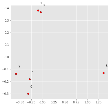
The SparkRecomendation.ipynb notebook used the Spark framework to apply SVD to reduce the dimensions of the matrix. As a result, the same model is represented in a dense form. Note that books or users which are correlated should be near each other in this new vector space. Figure 2 shows the position of some books after SVD dimension reduction. it’s possible to see that correlated items are near each other. 1 and 3 are classical books and 0 and 4 are self help books. However, in some examples the expected results are not what you’d expect when using common sense. 2 and 5 are books about philosophy and are not close to each other. Maybe, because one is more for common readers and the other for professionals.

Figure 1. Svd algorithm for dimension reduction.

Figure 2. Position of some books based on their dimensions after SVD reduction : 0 “Amigos e Influenciar Pessoas” ; 1 “dom casmurro”; 2 “O Que e Ideologia”, 3 “moreninha” , 4 “Quem Mexeu no Meu Queijo?” ; 5 “Convite a Filosofia:”
The notebook Similarity.ipynb used dense matrix representation, calculated by the previous notebook, to find the most similar books to each publication in the dataset. Below we can see some examples of the results:
- Memorias postumas de Bras Cubas: 1 Til; 2. A cidade e asFol serras; 3.Dom Casmurro;
- Como Fazer Amigos e Influenciar Pessoas: 1. Branding; 2. Almas Gemeas;
- HarryPotter e o calice de fogo : 1 Harry Potter e a Ordem da Fenix; 2 Harry Potter e o Enigma do Principe
In most cases, the results are not a surprise: Classical books are near classical books and best sellers are near best sellers. This is a good sign that the model has done a good job. However, some surprises have appeared, self help books are near management best sellers. This could be a sign that people who read self help books also read management best sellers.
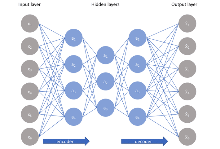
The Recomender_amazon_word2Vec.ipynb and Similarity.ipynb notebooks did the same dimensionality reduction process as done before, however istend of SVD they used auto encode provided by amazon SageMaker. Autoencoder is an artificial neural network algorithm. Figure 3 shows the auto encoder architecture. In the training phase, Autoencoder tries to find the weights which minimize the difference between the input layer and the output layer and the data in the middle of the model is the input in a dense form.
 The figure 3. A Schematic of Autoencoder.

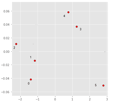
Figure 4. Position of some Items based on their dimensions after autoencoder dimension reduction : 0 “Amigos e Influenciar Pessoas” ; 1 “dom casmurro”; 2 “O Que e Ideologia”, 3 “moreninha” 4 “Quem Mexeu no Meu Queijo?” ; 5 “Convite a Filosofia:”
Using the autoencoder results, we have calculated the positions (figure 4) and the nearest neighborhood of the the same examples used in SVD,:
- Memorias postumas de Bras Cubas: 1. Nada dura para sempre; 2. Indomada: 3. A Ilha perdida
- Como Fazer Amigos e Influenciar Pessoas: 1. Amar verbo intransitivo: 2. Diamantes do Sol
- HarryPotter e o calice de fogo : 1. Harry Potter e o Enigma do Principe: 2. Harry Potter e as Relíquias da Morte:
The used SVD and Autoencoder models are different in their conception. AutoEncoder uses a sequence of items as input and the SVD model uses a correlated matrix. SVD works with linear relationships and autoencode works with liner and non-linear relationships. Thus it is not possible to compare the two algorithms using error functions. However, if we compare the results using human common sense, SVD looks more similar to what we would expect, with similar items with the same subject being closer to each other.
