A New Class of Non-standard Probability Distributions

The probability distributions introduced in this article generalize what is known as infinite convolutions of centered Bernoulli or Rademacher distributions. Some of them are singular (examples are provided), and these probability distributions have an infinite number of parameters, resulting in unidentifiable models. There is an abundant literature about particular cases, but typically quite technical and hard to read. Here we describe more diverse models including generalized random harmonic series, yet in simple terms, without using advanced measure theory. The concept is rather intuitive and easy to grasp, even for someone with limited exposure to probability theory. 

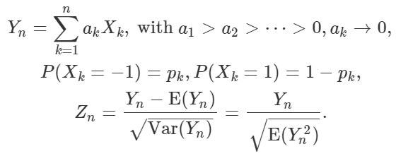
The distributions presented here are associated with a sum of independent random variables defined as follows:

Here pk = 1/2. The parameters are the ak‘s. We are interested in the case where n is infinite. Of course, all the odd moments are zero due to symmetry, thus E(Yn) = 0. We are especially interested in the distribution of the normalized variable Zn. When n is infinite, the generally continuous support domain can be infinite, finite, or fractal-like like (the Cantor set is a particular case). Of course the minimum (respectively the maximum) is achieved when all the ak‘s are – 1 (respectively +1), and these two quantities determine the lower and upper bounds of the support domain. Examples are discussed below. The uniform and Gaussian distributions are examples of limiting distributions, among many others. Numerous references are included.

1. Properties

Here MGF denotes the moment generating function, and CF denotes the characteristic function. Let

Then it is easy to establish the following:

The fourth and six moments are explicitly mentioned here, probably for the first time. They can be recursively derived from the MGF using the approach described here. The dominant term for the second, fourth, and six moments are respectively equal to 1, 3, and 15. This is obvious by looking at the above formula. Interestingly, these values 1, 3, and 15 (along with the fact that odd moments are all zero) are identical to those of a normal N(0,1) distribution. The Gaussian approximation generally holds when the variance for Yn becomes infinite as n tends to infinity.

The probability distribution depends only on An(r) for r = 2, 4, 6, and so on. So two different sets of ak‘s producing the same An(r)’s, result in the same distribution. This is important for statisticians using model-fitting techniques based on empirical moments, to check how good the fit is between observed data and one of our distributions. In some cases (see next section), the density function does not exist. However the cumulative distribution function (CDF) always exists, and the moments can be retrieved from the CDF, using a classical mechanism described here. Even in that case, the above formulas for the moments, are still correct.

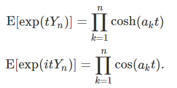
The MGF (top) and CF (bottom), for Yn, are:

Here cosh stands for the hyperbolic cosine. If ak = 2^k (2 at power k) then as n tends to infinity, the CF tends to (sin t) / t. This corresponds to the distribution of a random variable uniformly distributed on [-1, 1]. For details, see here. The CF uniquely characterizes the CDF.

2. Examples

I provide two examples: the classic infinite Bernoulli convolution, and the generalized random harmonic series.

2.1. Infinite Bernoulli convolutions

This case corresponds to ak = b^k (b at power k), with b  >  1. The case b = 2 was discussed in the last paragraph in section 1. If b = 2, it leads to a continuous uniform distribution for Zn as n tends to infinity. In the general case, since Var[Yn] is always finite, even if n is infinite, the Central Limit Theorem is not applicable. The limiting distribution can not be Gaussian. Also, the support domain of the limiting distribution is always included in a compact interval. However, if both b tends to 1, and n tends to infinity, then the limiting distribution for Zn is Gaussian with zero mean and unit variance. I haven’t fully proved this fact yet, so it is only a conjecture at this point. The closer you get to b = 1, the closer you get to a bell curve.

There are three different cases:

• b = 2: Then the first n terms of the random binary sequence (Xk) are equivalent to the first n binary digits of the (uniformly generated) number (Yn + 1)/2 if you replace Xk = -1 by Xk = 0. This also explains why the limiting distribution of Yn is uniform on [-1, 1]. 
• b  >  2: This is when the limiting distribution is always singular, and there is a simple explanation to this. Let’s say b = 3. Then instead of dealing with base 2 as in the previous case, we are generating random digits (and thus numbers) in base 3. But we are generating numbers that can not have any digit equal to 2 in base 3. In short, we are generating a small, very irregular subset of all potential numbers between the minimum -1/2 and the maximum 1/2. The support domain of the limiting distribution of Yn is equivalent to the Cantor set: see here for details; it is a small subset of [-1/2, 1/2] if b – 3. See also here.
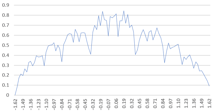
• 1  <  b  < 2: One would expect that the limiting distribution is smooth and continuous on a compact support domain. Indeed this is almost always the case except for particular values of b such as Pisot numbers.  One such example is b = (1 + SQRT(5))/2, known as the golden ratio. The limiting distribution is singular, and the CDF is nowhere differentiable, so the density does not exist. See the picture below. See also here and here.

Figure 1: Attempt to show how the density would look like if it existed, when b is the golden ratio

For other similar distributions, see my article on the Central Limit Theorem, here, or chapter 8, page 48, and chapter 10 page 63, in my recent book, here. See also here, where some of these distributions are called Cantor distributions, and their moments are computed. The case when pk (introduced in the first set of formulas in this article) is different from 1/2, can also lead to Cantor-like distributions. An example, leading to a Poisson-Binomial distribution, is discussed here.

2.2. Generalized random harmonic series

This case corresponds to ak = k^s (k at power s) with s  >  0. The most well-known case is when s = 1, thus the name random harmonic series. It has been studied, for instance here. It can be broken down in three sub cases:

• s  <  1/2: In that case, Var[Yn] is always infinite and the limiting distribution for Zn is Gaussian with zero mean and unit variance.
• s = 1/2: This is a special case. While Var[Yn] is still infinite, it is not obvious that the limiting distribution of Zn is still Gaussian. In particular, we are dealing with non identically distributed terms in the definition of Yn, so the Central Limit Theorem must be handled with care. But a proof of asymptotic normality, based on the Berry-Esseen inequality, can be found here. 
• s  >  1/2: Here Var[Yn] is finite. We are dealing with a smooth continuous distribution at the limit, with a compact support domain, and thus non-Gaussian. This case is strongly connected to the Riemann Zeta function. For instance, if k = 1, the second, fourth and six moments, computed using the formulas in section 1, are

The first identity is well-known. More can be found here. If you allow s to be a complex number, the setting becomes closely related to the famous Riemann Hypothesis, see here. Other distributions related to the Riemann zeta function are discussed here.