New & Notable
Top Webinar
Recently Added

The key to conversational speech recognition
Jelani Harper | October 9, 2025 at 2:32 pmAdvancements in statistical AI applications for understanding and generating text have been nothing short of staggering ...
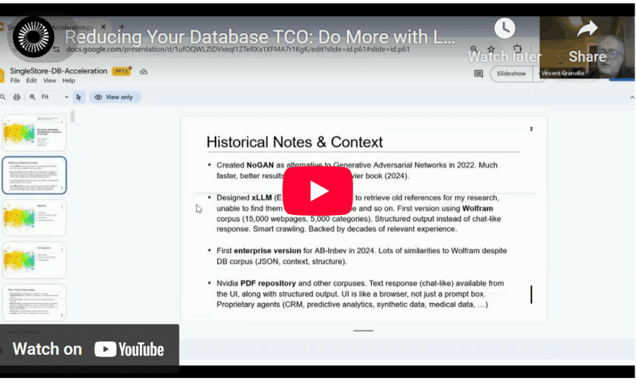
How to Get AI to Deliver Superior ROI, Faster
Vincent Granville | October 1, 2025 at 3:59 amReducing total cost of ownership (TCO) is a topic familiar to all enterprise executives and stakeholders. Here, I discus...
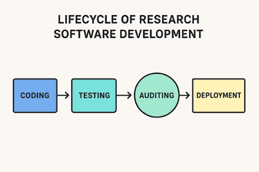
Code audits in R&D-driven applications
Edward Nick | September 24, 2025 at 12:37 pmWriting software for research isn’t like making a shopping app. It often controls lab instruments, runs detailed simul...

Guide to freezing layers in AI models
Kevin Vu | September 24, 2025 at 12:34 pmMaster the art of freezing layers in AI models to optimize transfer learning, save computational resources, and achieve ...

Secrets of time series modeling: Nested cross-validation
Vlad Johnson | September 22, 2025 at 2:55 pmWelcome to the series of articles on the secrets of time series modeling. Today’s edition features the nested cross-va...

How business leaders are using AI to make data-driven decisions
Edward Nick | September 10, 2025 at 10:40 amIntuition alone is no longer enough for effective leadership in the modern business world. Business leaders increasingly...

The data platform debt you don’t see coming
Saqib Jan | August 28, 2025 at 2:05 pmData Platform Debt...
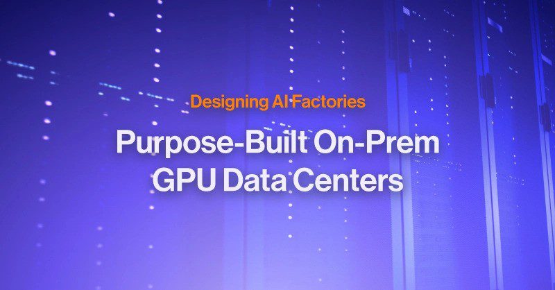
Designing AI factories: Purpose-built, on-prem GPU data centers
Martin Summer | August 26, 2025 at 2:39 pmDiscover how purpose-built AI factories are transforming on-premises GPU data centers for high-performance AI workloads,...

How diagnosis image annotation turns scans into insights
Rayan Potter | August 26, 2025 at 12:40 pmA radiologist looks at hundreds of CT images to find a tiny shadow that could be cancer. At these moments, every pixel m...

How AI shapes the future of work with superworkers
Tarique | August 26, 2025 at 9:04 amThe dialogue surrounding AI often raises anxiety: Will I be automated out of a job? The fact is, things are far more opt...
New Videos

Swiss Vault is bringing hyperscaler power to everyone
Interview with Bhupinder Bhullar In a world increasingly dominated by AI, massive data creation, and energy-hungry compute infrastructure, the question isn’t just how to store…
A/B Testing Pitfalls – Interview w/ Sumit Gupta @ Notion
Interview w/ Sumit Gupta – Business Intelligence Engineer at Notion In our latest episode of the AI Think Tank Podcast, I had the pleasure of sitting…
Davos World Economic Forum Annual Meeting Highlights 2025
Interview w/ Egle B. Thomas Each January, the serene snow-covered landscapes of Davos, Switzerland, transform into a global epicenter for dialogue on economics, technology, and…