Exploring foundational machine learning algorithms: Linear regression, decision trees, and K-nearest neighbors

Machine learning algorithms power predictive modeling and data analysis. Linear regression, decision trees, and k-nearest neighbors enable limitless possibilities. This article explores their principles and applications, inspiring machine learning creativity.

Exploring Linear Regression

Understanding the basics

The best line for a set of data points is the goal of linear regression. It is assumed that there is a linear relationship between the predictors and the response in linear regression. Fitting a line involves adjusting its slope and intercept to minimize the sum of the squares of the differences between observed values and line predictions.

Consider the following simple dataset table to illustrate this idea:

In this basic example, the test score (Y) increases with the number of hours studied (X), suggesting a linear relationship. Linear regression models this relationship to predict Y for any X.

Linear regression is elegantly simple and interpretable. It is a good starting point for machine learning model dynamics.

The algorithm is simple but has major implications. It underpins more complex models and permeates machine learning.

As we implement linear regression in Python, we’ll see how these basics work with real data and can be extended to handle more complex scenarios.

Implementing in Python

After understanding linear regression theory, the next step is to apply it. Python is ideal for such projects due to its rich library ecosystem.

Linear regression is usually implemented using scikit-learn, which is simple and efficient. Steps are summarized here:

1. Import necessary libraries

Import the necessary libraries first. Sklearn provides functions for splitting the dataset and linear regression, while numpy performs numerical operations.

import numpy as np

from sklearn.model_selection import train_test_split

from sklearn.linear_model import LinearRegression

from sklearn.metrics import mean_squared_error, r2_score

2. Split data into training and testing sets

Load your dataset into a Pandas DataFrame before running this code. Assume your dataset is in df and you want to predict ‘target’.

# Assuming your dataset is a Pandas DataFrame named `df`

# X represents the features, while y is the target variable

X = df.drop(‘target’, axis=1)  # drop the target variable from the dataset to isolate features

y = df[‘target’]  # the target variable

# Split the dataset into training (70%) and testing (30%) sets

X_train, X_test, y_train, y_test = train_test_split(X, y, test_size=0.3, random_state=42)

3. Create and train linear regression model

Next, we fit a LinearRegression model to our training data.

# Create linear regression object

regressor = LinearRegression()

# Train the model using the training sets

regressor.fit(X_train, y_train)

4. Evaluate the model

We evaluate the model’s performance using metrics like MSE and R² score after making predictions on our test set.

# Make predictions using the testing set

y_pred = regressor.predict(X_test)

# The mean squared error

mse = mean_squared_error(y_test, y_pred)

print(f”Mean squared error: {mse}”)

# The coefficient of determination: 1 is perfect prediction

r2 = r2_score(y_test, y_pred)

print(f”Coefficient of determination: {r2}”)

The following steps will create a basic linear regression model for your dataset. These blocks require the sklearn and numpy libraries and a Pandas DataFrame with your dataset loaded and preprocessed (if needed).

The above steps give a broad overview, but the details matter. Parameter tuning and data preprocessing can improve the model’s predictive power. An astute practitioner will find the process meticulous but rewarding.

Handling multivariate data in linear regression

In machine learning, multivariate data involves a complex dance of variables that can affect model performance. Aligning data from different sources is like conducting an orchestra, where each instrument’s timbre must match. We coordinate this alignment using feature concatenation, extraction, and tree and metric-based learning.

In the pursuit of machine learning’s promise, missing data must be considered. This phantom can degrade our datasets and bias our models. Our best defense is meticulous data collection, which accounts for and accurately represents each variable.

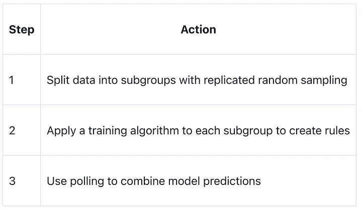
High variance is another major issue. The bagging algorithm replicates sampling to divide data into subgroups. This process uses a training algorithm to create diverse rules and polling to combine predictions. The following table outlines high variance mitigation steps:

Data quality is the foundation of machine learning. The complexity of managing many input variables in different formats requires a strategic approach to identifying, collecting, and managing them. We can only ensure data integrity and utility through careful planning, enabling insightful and robust machine-learning models.

Decoding decision trees

Tree structure

Elegant and powerful structure underpins decision trees. Each internal node represents a ‘test’ on an attribute, each branch represents the result of the test, and each leaf node represents a class label (which is chosen after computing all of the attributes). Paths from root to leaf represent classification rules.

Decision trees repeatedly split data into subsets based on the best attribute at each level. A simplified binary decision tree:

• All of the data in the dataset is represented by the root node.
• Decision Node: Conditional data splitters.
• Leaf Node: Class-label terminal nodes that predict outcomes.

Decision trees are easy to understand and interpret because they mimic human decision-making.

The algorithm used to determine the ‘best’ attribute at each decision node is crucial. Gini impurity or information gain for classification trees and variance reduction for regression trees are used. Algorithms greatly affect tree performance and complexity.

Pruning techniques

The lush garden of decision trees requires artful pruning to prevent complexity from overfitting.

Pruning removes branches that don’t affect the final decision, simplifying the model without compromising accuracy. Statistical infographics help visualize how pruning affects decision tree structure.

The two main pruning methods are:

• If further splitting is pointless, pre-pruning (Early Stopping) stops tree growth.
• After full tree growth, it removes branches with low predictive power (Cost Complexity Pruning).

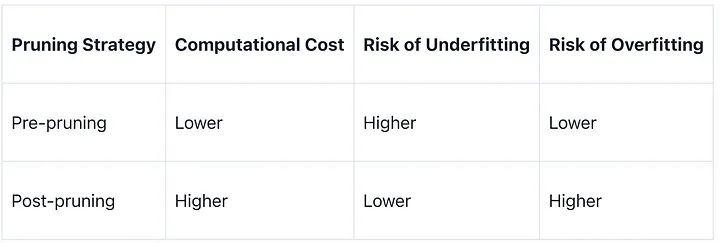
Each method has pros and cons, depending on the dataset and desired model complexity and predictive performance. Pre-pruning may save computational resources but underfit the data due to conservatism. However, post-pruning is more thorough but computationally intensive. The table below summarizes these trade-offs:

In conclusion, strong decision trees require careful pruning. It requires knowledge of the tree’s structure and the dataset’s nuances to strike a delicate balance.

Ensemble methods in decision trees

After learning about decision trees, ensemble methods are intriguing. Ensemble learning combines multiple models’ wisdom to create a more accurate and reliable prediction system. This is like consulting a panel of experts rather than one. Ensembles excel at complex problems like sentiment analysis, improving performance metrics.

Ensemble methods are a strategic synthesis of diverse models, each contributing its own perspective to the final decision.

Popular model aggregation methods include majority voting, which balances simplicity and effectiveness. However, model selection and combination require a deep understanding of the problem. Ensemble methods include bagging, boosting, and stacking, each with their own benefits and uses.

Ensemble methods demonstrate the power of collaboration in machine learning, where no algorithm is supreme. They show us that diversity is strong.

Unveiling K-nearest neighbors

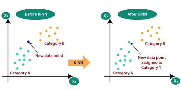
Machine learning’s K-nearest neighbors (KNN) algorithm is powerful and versatile. This is widely used for classification and regression, revealing new insights from data sets and improving prediction accuracy. KNN helps us spot patterns and relationships by assuming similar things are nearby. KNN lets us explore hidden data and learn new things to solve problems and understand the world. KNN’s basic operation:

1) Number of Neighbours (K): Choose K nearest neighbors to consider. Tweak this hyperparameter for better performance. A small K provides the most flexible fit, with low bias and high variance, while a larger K smooths the decision boundary, with lower variance and higher bias.

2) Distance Metric: Calculate point distances to find nearest neighbors. Next, we discuss their distance types. Depending on the data, the distance metric can significantly impact model performance.

Distance metrics

The distance metric used in K-Nearest Neighbors (KNN) can greatly affect model performance. The distance metric determines how ‘nearness’ is calculated between data points, so choosing the right one is like choosing the right lens for our data.

• Most common and intuitive metric: Euclidean Distance, measuring straight-line distance between two points.
• Manhattan Distance: Sum of absolute coordinate differences for grid-like path planning.
• For categorical data, Hamming Distance counts the number of positions where the symbols differ.
• Useful in text analysis, cosine similarity measures the angle between two vectors.

Each metric has pros and cons, so a combination or custom metric may be best. Choice should be based on dataset characteristics and model application.

Choosing the right ‘K’

The optimal ‘K’ in K-Nearest Neighbours (KNN) is a delicate balance between underfitting and overfitting. The granularity of the classification or regression task depends on the ‘K’ chosen. Overfitting can result from a smaller ‘K’ making the model sensitive to noise, while underfitting from a larger ‘K’ smoothing predictions too much.

Consider these ‘K’ selection strategies:

Use cross-validation to evaluate the model with different ‘K’ values.

The ‘K’ with the lowest validation error rate is often best.

Start with the square root of the number of data points and adjust based on performance.

Remember that the best ‘K’ is subjective. This parameter should be tailored to the dataset and problem context.

Impact of outliers in K-nearest algo

Outliers can significantly skew k-nearest neighbors (KNN) algorithm results, resulting in less accurate predictions. Outliers is data that deviates significantly from the overall pattern, and the KNN algorithm may use misleading information when making decisions.

KNN relies on neighboring points, so outliers are especially noticeable. An outlier can drastically change a point’s neighborhood, causing a misclassification or regression error.

Several methods can reduce outliers:

• Cleaning: Remove data entry and measurement errors that caused outliers.
• Use median and interquartile range scaling to reduce outlier sensitivity.
• Adjustments: Weight neighbors by distance to reduce outliers in the KNN algorithm.

To determine whether outliers are anomalies that should be excluded or valuable extremes that enrich the dataset, a thorough analysis is needed. The dataset context and analysis goals should guide outlier adjustment or removal.

Conclusion

In conclusion, linear regression, decision trees, and k-nearest neighbors are essential machine learning algorithms for predictive modelling and data-driven decision making.

These algorithms lay the groundwork for machine learning principles and are essential for beginners and experts.

Mastering these algorithms allows one to create innovative solutions and advance artificial intelligence. These foundational algorithms form the basis for more complex models and techniques as we explore machine learning, enabling exciting AI advances.