
“Thus learning is not possible without inductive bias, and now the question is how to choose the right bias. This is called model selection.” ETHEN ALPAYDIN (2004) p33 (Introduction to Machine Learning)
There are many more definitions concerning Model Selection. In this article, we are going to discuss Model Selection and its strategy for Data Scientists and Machine Learning Engineers.
An ML model(s) are always constructed using various mathematical frameworks and that would generate predictions based on the nature of the dataset and finding patterns out of it.
Understand Machine Learning Model and Algorithm
Most of them are really confused between two terminologies in machine learning – ML-Model and ML-Algorithm. Even me too. But over the period I got to understand the thin line between these two terms. The understanding of these differences is very important during the machine learning life cycle.
An ALGORITHM is always RUN ON THE DATA to create a stabilized model.

The MODEL includes both the DATA and a PROCEDURE (algorithm). Which is using the data to predict a new set of data. The ML- Model usually represents that what was learned over time by the algorithm, which was run on the data. We could say that the model is a packed item after all learning processes and to make predictions in future with new data.

Model Selection is a mantra
Always selection is the process of selecting the best one by comparing and validating with various parameters and choosing the final one. So in machine learning as well the model selection is not an exceptional case either way!
In Data Science and ML world, this is coming under the collection of available algorithms under different names, purposes, nature of the data. After applied on the training dataset, followed by selecting the BEST ONE and promoting the same model into the PRODUCTION for the live/streaming dataset and monitoring the outcome. And on top make sure the best results and sustaining with the same model for new data for regression, classification and clustering problem statements.
Model Selection is one of the critical stages in the Data Science and ML life cycle and the process of selecting the best machine learning model ( data and algorithm combination)
Where is Model Selection in the ML life cycle?
After successful completion of the EDA and Feature Engineering process, we’re safer to start doing the model selection for the finetuned dataset with the following key considerations.
- Nature of the dataset
- Column collections
- Type of individual column/features
- Given problem statement(s).
Below lifecycle diagram representing the entire flow and is highlighted with the model selection area.
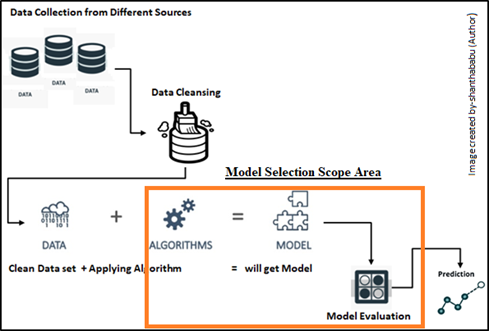
The highlight here is we may have a dataset and all preprocessing techniques and various machine learning nuances have been applied to it, but no concrete idea which model from classification or regression predictive model, etc.,
The bottom line is “We have to compare the relative performance between more than two models for the given and cleaned data set”
The model should be very flexible and fit into the data and explain the insight of the data in statistical estimation form.
Before we going for model selection, have to find out the level of data distributions and other dependency factors which are involved in the given dataset. These factors are commonly known as bias and variance. Let’s discuss how these factors impact model selection.
During the model selection, we are supposed to get ready with the required sufficient data in hand. In an ideal situation, we have to split the data into three different sets of data
- Training set
- Used to fit the models
- Validation set
- Used to Estimate the prediction of error for the model
- Test set
- Used for Assessment of the Generalization error
Once all the above process flow has been completed the final model could be select from the list of models.
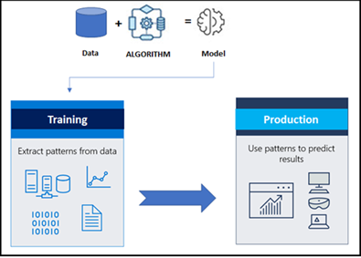
What is Bias and Variance, How it playing in Model selection?
Bias: Bias is an error that has been introduced in our model due to the oversimplification of used the machine learning algorithm. The basic problem here is that the algorithm is not strong enough to capture the patterns or trends in the fine-tuned data set. The root cause for this error is when the data is too complex for the algorithm to understand. so it ends up with low accuracy and this leads to underfitting the model.
Generally below are the list of algorithms leading to low bias
- Decision Trees
- k-NN and
- SVM
And high bias leading machine learning algorithms are as below
- Linear Regression
- Logistic Regression
Variance: Variance is an error that has been introduced in our model due to the selection of a complex machine learning algorithm(s), with high noise in the given dataset, resulting in high sensitivity and overfitting. You can observe that the performs of the model is well on the training dataset but poor performance on the testing dataset.
The below visualization depicting the relation between Bias and Variance
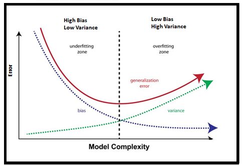
You can observe from the above visualization, that the model complexity has increased after a certain point, your model becomes overfitting.
we have to keep it in our mind is “Increasing the bias will decrease the variance. Increasing the variance will decrease bias, So Bias and Variance are indirectly proportional to each other.
Types of Model Selection
There are 2 major techniques in model selection, as mentioned earlier this is a mathematical model and patterns are extracted from the given dataset.
- Resampling
- Probabilistic
Resampling: These are simple techniques just rearranging data samples and inspecting that the model performs good or bad with the data set.
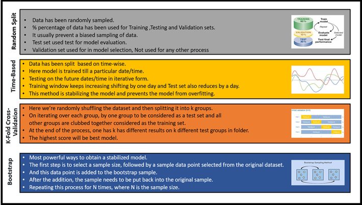
Let’s focus on few samples now, to understand the concepts, that we have discussed above.
I.Bias & Variance
The below code tells you
print(“############################################”)
print(” Importing required library “)
print(“############################################”)
import mlxtend
from pandas import read_csv
from sklearn.model_selection import train_test_split
from sklearn.linear_model import LinearRegression
from mlxtend.evaluate import bias_variance_decomp
# load dataset
print(“############################################”)
print(” Data Loading “)
print(“############################################”)
dataframe = read_csv(“housing.csv”)
data = dataframe.values
X, y = data[:, :-1], data[:, -1]
print(X)
print(“#######################################################”)
print(” Spliting the data for test and train “)
print(“#######################################################”)
X_train, X_test, y_train, y_test = train_test_split(X, y, test_size=0.25, random_state=1)
print(“#######################################################”)
print(” Applying LinearRegression “)
print(“#######################################################”)
model = LinearRegression()
# Estimating Bias and Variance bias_variance_decomp
print(“#######################################################”)
print(“Estimating Bias and Variance using Bias Variance Decomp”)
print(“#######################################################”)
mse, bias, var = bias_variance_decomp(model, X_train, y_train, X_test, y_test, loss=’mse’, num_rounds=200, random_seed=1)
print(“############################################”)
print(‘Mean Squared Error (MSE): %.2f’ % mse)
print(‘Bias of the given data: %.2f’ % bias)
print(‘Variance of the given data: %.2f’ % var)
print(“############################################”)
Output
############################################
Importing required library
############################################
############################################
Data Loading
############################################
[[2.7310e-02 0.0000e+00 7.0700e+00 … 1.7800e+01 3.9690e+02 9.1400e+00]
[2.7290e-02 0.0000e+00 7.0700e+00 … 1.7800e+01 3.9283e+02 4.0300e+00]
[3.2370e-02 0.0000e+00 2.1800e+00 … 1.8700e+01 3.9463e+02 2.9400e+00]
…
[6.0760e-02 0.0000e+00 1.1930e+01 … 2.1000e+01 3.9690e+02 5.6400e+00]
[1.0959e-01 0.0000e+00 1.1930e+01 … 2.1000e+01 3.9345e+02 6.4800e+00]
[4.7410e-02 0.0000e+00 1.1930e+01 … 2.1000e+01 3.9690e+02 7.8800e+00]]
#######################################################
Spliting the data for test and train
#######################################################
#######################################################
Applying LinearRegression
#######################################################
#######################################################
Estimating Bias and Variance using Bias Variance Decomp
#######################################################
############################################
Mean Squared Error (MSE): 26.25
Bias of the given data: 25.08
Variance of the given data: 1.17
############################################
II.Random split
print(“############################################”)
print(” Random split “)
print(“############################################”)
print(“############################################”)
print(” Importing required library “)
print(“############################################”)
import numpy as np
from sklearn.model_selection import train_test_split
print(“############################################”)
print(” Creating array,reshaping and arraging “)
print(“############################################”)
X, y = np.arange(10).reshape((5, 2)), range(5)
print(“############################################”)
print(“y – values:”,list(y))
print(“############################################”)
print(“X – values:”,list(X))
print(“############################################”)
Output
############################################
Random split
############################################
############################################
Importing required library
############################################
############################################
Creating array,reshaping and arraging
############################################
############################################
y – values: [0, 1, 2, 3, 4]
############################################
X – values: [array([0, 1]), array([2, 3]),
array([4, 5]), array([6, 7]), array([8, 9])]
############################################
III. KFold
K-Fold
############################################
############################################
Importing required library
############################################
############################################
Defining array
############################################
############################################
No. Of Fold in the given array
############################################
KFold(n_splits=4, random_state=None, shuffle=False)
TRAIN: [1 2 3] TEST: [0]
TRAIN: [0 2 3] TEST: [1]
TRAIN: [0 1 3] TEST: [2]
TRAIN: [0 1 2] TEST: [3]
IV. Bootstrapping with Array
Output
############################################
Bootstrapping with Array
############################################
############################################
Importing required library
############################################
############################################
Loading sample.csv file
############################################
############################################
Top 5 records from dataset
############################################
Hours Calories Weight
0 1.0 2500 95
1 2.0 2000 85
2 2.5 1900 83
3 3.0 1850 81
4 3.5 1600 80
############################################
Defining Target Variable – Weight
############################################
[95 85 83 81 80 78 77 80 75 70]
#################################################
Defining Predictor Variables – Hours & Calories
#################################################
[[1.00e+00 2.50e+03]
[2.00e+00 2.00e+03]
[2.50e+00 1.90e+03]
[3.00e+00 1.85e+03]
[3.50e+00 1.60e+03]
[4.00e+00 1.50e+03]
[5.00e+00 1.50e+03]
[5.50e+00 1.60e+03]
[6.00e+00 1.70e+03]
[6.50e+00 1.50e+03]]
#################################################
Let’s perform Bootstrapping – Using simple loop
#################################################
###########################################################
Increasing the seed value for each iteration and building
DecisionTreeRegressor modle
###########################################################
#################################################
Bootstrapping trials :
List of Accuracy: [94.0, 95.0, 98.0, 98.0, 93.0]
#################################################
Final Average(Mean) accuracy 95.6
What is Model Evaluation Metrics in machine learning?
The straightforward answer is to evaluate the performance of the machine learning model which we have selected in the previous steps. The objective is to estimate the accuracy of a model on future (or) unseen data, So the model should be generalized form. Without performing this evaluation step(s), we shouldn’t move the model into production on unseen data. otherwise, we end up with a poor prediction, classification and etc.,
“We could say that the MODEL have to train such a way to Learn, but not to Memorize
Generalization of the model is the key takeaway
Guys! I trust you got some understanding from this article regarding “Machine Learning Model Selection & Evaluation Strategy”. I have tried to cover as quickly as possible without getting too much time. Thanks for your time in reading this. Hope it was useful. I will get back to you with a new and interesting topic. Until then, Cheers! Shanthababu,
