After being confined for 2 months and hearing the word pandemic almost daily, seeing graphs, opinions, time lines and values that rise and fall, I became curious. Firstly, what is a pandemic? Is it the same as an epidemic? A plague? Was the plague an epidemic? What do epidemiologists study? Yes, they study a discipline called epidemiology.
What is epidemiology?
Epidemiology studies the distribution, frequency, relationships, predictions, and control of all factors related to health and disease in the human population. Epidemiology has more to it, there is descriptive epidemiology, which as you can imagine focuses in recording and observing all the possible information in order to generate a hypothesis, there is also, analytical epidemiology, which is in charge of using statistical and probabilistic tools to search for relationships among the factors to which a population and disease are exposed, there is also experimental epidemiology, which is based on experimental studies generally on animals, eco-epidemiology, similar but in the field of ecology, and theoretical epidemiology, based on mathematic models.
Now I think we can already talk about what an epidemic actually is, right? Wikipedia defines it very well, saying that it is what happens when a disease affects more people than expected during a certain period of time. Well, when an epidemic spreads to different geographical regions it is called a pandemic. At least I already have something clear, I have even looked for examples of epidemics, for example:
- Smallpox – It is the pandemic that has caused the most deaths in all of history, and has left millions of people disfigured. The last case was in Somalia, in 1977.
- Measles – Second in the ranking, without eradicating, but at least we can prevent contagion.
- The Spanish Flu – Very concentrated, this pandemic operated between 1918 and 1920. As I have read, the name was given to us as it was the first country to report this epidemic.
- Typhus – From the 18th century, it is controlled.
- Cholera – It has 3 major pandemics, XIX and XX centuries. It still exists.
- The Black Plague – One of the most fatal epidemics of the human history. From the 14th century and the last outbreak in the 18th century.
- AIDS (HIV) – This disease is not the direct cause of death, but it weakens the immune system so much that almost any disease, however slight, can end a person’s life. Supposedly without a cure, it appeared in 1982.
- Ebola – The first epidemic outbreak dates from 1976, with fatality figures of over 80%, killing 2,830 people in Zaire and Sudan.
And in this last, more recent century, we have the epidemics of influenza A, the Zica virus and the current pandemic that we are going through, that of COVID-19.
The importance of epidemiology and mathematical models
For it was Daniel Bernoulli who published in 1760 the first article based on a mathematical application to an infectious disease, Smallpox. Soon after, d’Alembert continued his work and was the first to describe what the spread of disease was like using a model. A curiosity, Ronald Ross, 1902 Nobel Prize winner, showed that eliminating mosquitoes would end malaria.
It was not until 1927 when Kermack and McKendrick published a model to predict the final size of an epidemic, how it spreads, and what is known as the threshold theorem, which has been one of the most important contributions of theoretical epidemiology. This theorem basically came to tell us that the introduction of a highly infectious case in a susceptible community might not give rise to an outbreak or an epidemic, if the density of susceptibles is less than a certain critical value. Then we will go into more detail.
I wanted to highlight the importance of mathematical models when we speak in the field of health and diseases, since historically epidemics are one of the great fears for all people, since they completely isolated the population that suffered from it. This importance is mainly due to the fact that they show us causal relationships that are not easily observable at first sight, we can use mathematical models to predict the consequences and allow us to understand how a disease spreads through a population under multiple scenarios.
Epidemiological models
First of all, I want to remind you that we should not forget at any time that we are treating biological processes, that is, before a disease that is transmitted through an agent (rats, for example) we can formulate a model as if that disease were transmitted between humans. We might even believe that by quarantining infected individuals we could curb the disease, as happened in the city of Eyam in 1965 with the bubonic plague. What happened is that rats continued to spread the disease throughout England.
We can say that there are different factors within a disease that make it impossible to study all diseases in the same way. These factors can be the mode of transmission, infectious agents, the affected population and the states through which an individual can pass.
Transmission mode
It can be person to person like HIV or COVID-19, by the environment like cholera or by agents (insects) like malaria. It varies according to the disease.
Infectious agents
These are microorganisms capable of producing an infection or an infectious disease, for example, Viruses, Bacteria, Worms, etc. These agents condition the various states through which those affected by a disease pass.
The affected population
You have to study if you have immigration, emigration, births or deaths, etc.
The different states that an individual can go through
As I said before, the states are not the same for all diseases, but the following are usually used:
- S: Healthy and susceptible individuals to be infected.
- E: Latent-phase infected individuals (i.e. individuals infected who cannot infect others).
- I: Infected and infectious individuals who can infect others.
- A: Individuals resistant to the disease (usually after recover from illness or after being vaccinated)
- M: Individuals with temporary immunity to the disease (for example, inherited from the mother).
We usually consider that the population size is normalized, it is that is, the population has size 1. Therefore, each state represents the proportion of individuals in that state with respect to the total number of individuals in the population.
We have: S + E + I + R + M = 1
Types of diseases
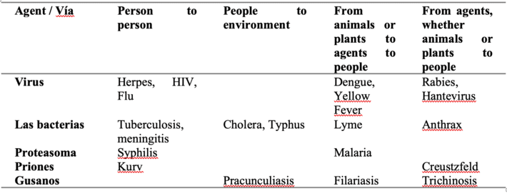
Types of mathematical models in epidemics
There are three types of models:
- Stochastics or focused on individuals, which come from the beginning of the 20th century, where a variable is taken as a random datum and the relationships between the variables are taken by means of probabilistic functions. They can be used in populations of any size.
- The deterministic or state-centered, from the 19th century, in which individuals belonging to a state of the model are considered as a whole and not individually. They can be used with large populations and facilitate analytical study of the epidemic.
- The hybrid models, which are obviously combined between a deterministic and a stochastic part.
Epidemic or endemic
We have to know how to differentiate between epidemic and endemic, one of the most important factors to study is whether or not that epidemic will be endemic.
To find out, we analyze the indicator R_0. R_0 is the basic breeding number, and consists of the average number of secondary infections that occur when an infectious individual (known as patient zero) is introduced into a susceptible population. In Christian, how many individuals will patient zero directly infect.
This value of R_0 is fundamental in epidemiology, since it tells us if the infection is going to spread, if R_0 <1 will disappear and if R_0> 1 we are facing an epidemic case:
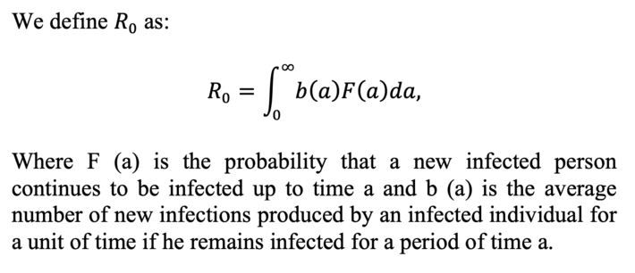
SIR model for epidemics
There is a vast literature on mathematical models that help predict whether or not an epidemic will spread. By going to a basic but functional one, we are going to focus on the SIR model, which as you may have imagined, the S is Susceptible to contract the disease, the I is for the Infected and the R for the Recovered.
If we define instant t, we can define:
- S (t) as the number of people susceptible to contracting the disease at time t.
- I (t) as the number of infected at time t.
- R (t) as the number of recovered at time t.
This model will consider two parameters, which are:
- β is the average number of contacts.
- γ the number of recovered divided by the total number of infected (rate of infected to recovered).
Thus, we can define the rate of passing from susceptible to infected as the average number of contacts for the probability of being infected (at time t):
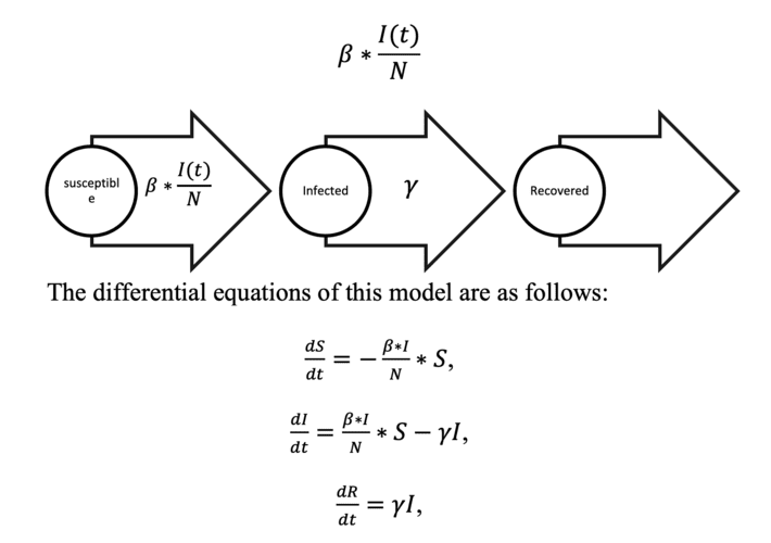
That is, the variation of susceptibles in t is the pass rate of susceptible to infected (in negative, since it decreases if the rate of infected increases) by the total number of susceptibles.
The variation of infected is the rate from susceptible to infected by the total number of susceptible (those infected increase) minus the transition rate from infected to recovered by the total of infected.
Finally, the recovery rate, as we have defined, would simply be the transition rate from infected to recovered by the total number of infected.
Thanks to the fact that the number of susceptibles plus the number of infected plus the number of recovered remains constant and is the total population, that is:
S(t)+I(t)+R(t)=N
dS/st + dI/dy + dR/dt=0
Then R (t) = N-S (t) -I (t) so the system with three equations becomes a system of two equations.
On the other hand, the solution S (t) can be obtained if we divide the first equation by the last one and integrate,

To the value β/γ we call it the basic reproduction number, which is the famous coefficient R_0.
This coefficient is very important for the study of the infected, since we can rewrite the equation in this way,

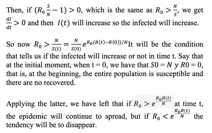
Let’s suppose t_1,…,t_n we got S(t_i ),I(t_i ) y R(t_i). So in order to estimate R_0 we substitute in S(t):
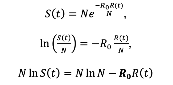
We can see that there is a linear relationship between the variables N lnS (t) = Y and R (t) = X since N lnN is constant.
Once we have calculated R_0 through this regression line and confirming a good fit with R ^ 2 we will be able to see if the value of R_0 e is greater or less than e^((R_0 R(t))/N) at some point t and conclude whether the infection will continue to expand or otherwise decrease. This R_0 is visually the slope of that regression line.
As the SIR model is one of the most basic that does not take into account the number of deaths, I advise that if used, that they be added to the number of infected, so we maintain the N of the population and assume that there are no births.
In one of the practices of the course “Learn to analyze COVID-19 data with R and Python” we are asked to calculate R_0 and comparing it with e^((R_0 R(t))/N) for the Community of Madrid. Well, as of May 12, 2020, when we are talking in terms of whether it is early or not to go to phase I in the Community of Madrid, with this simple SIR model the result is as follows:
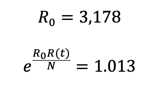
Now that R_0 is sufficiently greater than e^((R_0 R(t))/N), We can say that the virus is still spreading, so we still have to focus our attention (R^2=0,98).
References:
http://www.mat.ucm.es/~ivorra/papers/Diego-Epidemiologia.pdf
https://biblioteca.unirioja.es/tfe_e/TFE002211.pdf
https://es.wikipedia.org/wiki/Modelaje_matem%C3%A1tico_de_epidemias…
https://www.agenciasinc.es/Reportajes/Un-modelo-un-teorema-y-teoria…
Read more here.
