Quality inspection in manufacturing using deep learning based computer vision

Author: Partha Deka and Rohit Mittal

1. Introduction

Automation in Industrial manufacturing:

Today’s increased level of automation in manufacturing also demands automation of material quality inspection with little human intervention. The trend is to reach human level accuracy or more in quality inspection with automation. To stay competitive, modern Industrial firms strive to achieve both quantity and quality with automation without compromising one over the other.

Deep Learning for Quality inspection:

To meet industry standards quality inspectors in manufacturing firms inspect product quality usually after the product is manufactured, it’s a time consuming manual effort and a rejected product results in wasted upstream factory capacity, consumables, labor and cost. With the modern trend of Artificial Intelligence, industrial firms are looking to use deep learning based computer vision technology during the production cycle itself to automate material quality inspection. The goal is to minimize human intervention at the same time reach human level accuracy or more as well as optimize factory capacity, labor cost etc. The usage of deep learning is varied, from object detection in self-driving cars to disease detection with medical imaging deep learning has proved to achieve human level accuracy & better.

What is deep learning?

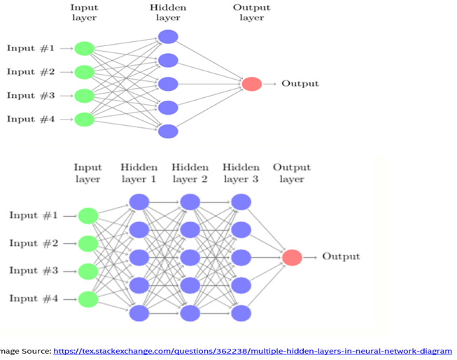
Deep learning is the field of learning deep structured and unstructured representation of data. Deep learning is the growing trend in AI to abstract better results when data is large and complex. Deep learning architecture consists of deep layers of neural networks such as input layer, hidden layers, and output layer. Hidden layers are used to understand the complex structures of data. A neural network doesn’t need to be programmed to perform a complex task. Gigabytes to terabytes of data are fed to the neural network architecture to learn on its own. Sample deep neural networks below:

Convolution neural Network:

Convolution neural network is a class of deep neural network commonly applied in image analysis. Convolution layers apply a convolution operation to the input passing the result to the next layer. For example an image of 1000 by 1000 pixels has 1 million features. If the first hidden layer has 1000 neurons, it ends up having 1 billion features after the first hidden layer. With that many features, its difficult to prevent a neural network from overfitting with less data. The computational and memory requirements to train a neural network with a billion features is prohibitive. The convolution operation brings a solution to this problem as it reduces the number of free features, allowing the network to be deeper with fewer features. There are two main advantages of using convolution layers over fully connected layers – parameter sharing and sparsity of connections.

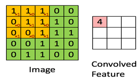
Convolution neural network look for patterns in an image. The image is convolved with a smaller matrix and and this convolution look for patterns in the image. The first few layers can identify lines / corners / edges etc, and these patterns are passed down into the deeper neural network layers to recognize more complex features. This property of CNNs is really good at identifying objects in images.

Convolution neural network (aka ConvNet) is nothing but a sequence of layers. Three main types of layers are used to build ConvNet architectures: Convolutional Layer, Pooling Layer, and Fully-Connected Layer. These layers are stacked layers to form a full ConvNet architecture:

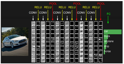
Image Source: http://cs231n.github.io/convolutional-networks/

The below image clarifies the concept of a convolution layer:

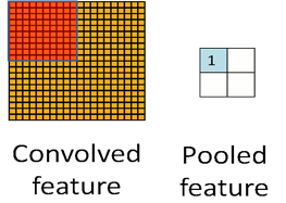
The below image clarifies the concept of a pooling layer (Average or Max pooling):

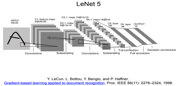
Following is one of the original CNN architectures:

Visualizing CNN:

Following is an image of a crack on a plain surface:

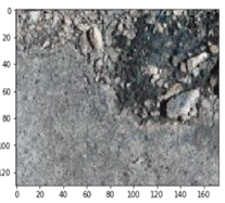
Two layers each of Conv (one 3X3 filter), ReLU and Max Pooling (2X2) similar to LENET-5 architecture are applied to the crack image above. It can be seen below that the CNN architecture is focusing on the blocks of crack area and the spread of it throughout the surface:

2. Case Study – Introduction

To maintain confidentiality of our work we are presenting an abstract use case below:

Problem Statement:

Detecting bad quality material in hardware manufacturing is an error prone & time consuming manual process and results in false positives (detecting a bad one as good one). If a faulty component/part is detected at the end of the production line there is loss in upstream labor, consumables, factory capacity as well as revenue. On the other hand, if an undetected bad part gets into the final product there will be customer impact as well as market reaction. This could potentially lead to irreparable damage to the reputation of the organization.

Summary:

We automated defect detection on hardware products using deep learning. During our hardware manufacturing processes there could be damages such scratches / cracks which make our products unusable for the next processes in the production line. Our deep learning application detected defect such as a crack / scratch in milliseconds with human level accuracy and better as well as interpreted the defect area in the image with heat maps.

Details of our Deep Learning Architecture:

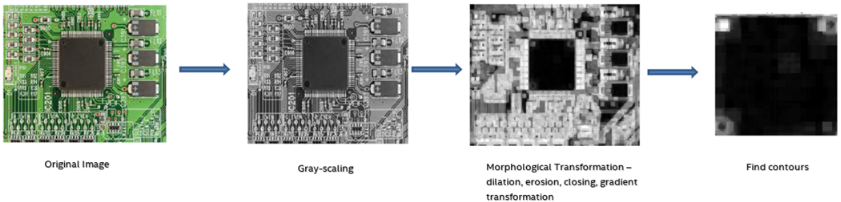
To describe things better, we are using an example image of a circuit board with an integrated chip on it below:

3. Case Study: Our first approach:

We adopted a combination of pure computer vision approach (non-machine learning methods) to extract the region of interest (ROI) from the original image and a pure deep learning approach to detect defects in the ROI.

Why ROI extraction before DL?

While capturing the images, the camera assembly, lighting etc. was focusing on the whole area of the circuit (example images below). We are only inspecting the chip area for defects and no other areas in the circuit. We found with a few experiments that DL accuracy increased substantially when neural networks focus only on the area of interest rather than the whole area.

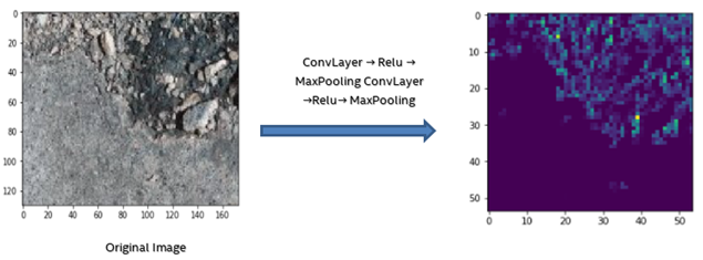
First Extract “Region of Interest (ROI)” with Computer Vision (Non-Machine Learning Methods). Here, we go through multiple processes on the image such as gray scaling, transformations such as eroding, dilating, closing the image etc. and eventually curve out the ROI from image based on use case type / product type etc. The basic idea of erosion is just like soil erosion – it erodes away the boundaries of foreground object. Dilating is just opposite of erosion – it increases the size of foreground object. Normally, in cases like noise removal, erosion is followed by dilation. Opening is just another name of erosion followed by dilation. It is useful in removing noise. Closing is reverse of opening, dilation followed by erosion. It is useful in closing small holes inside the foreground objects, or small black points on the object. Gradient transformation is the difference between dilation and erosion of an image. Overall, these steps help in opening up barely visible cracks / scratches in the original image. Refer the figure below :

Secondly, detect defects using deep neural networks(deep neural network (CNN)-Based Models) using proven CNN topologies such as Inception Net(aka Google Net), Res Net, Dense Net :

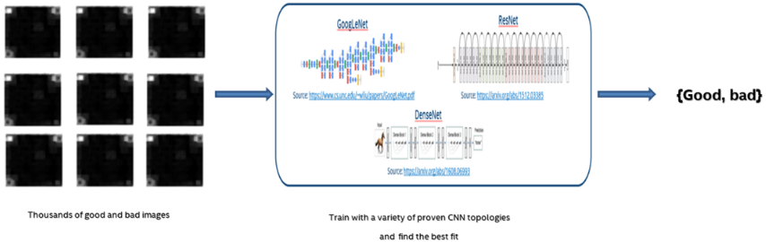
Some other areas where experimentation was necessary to find the optimal architecture

Data Augmentation: We have few thousand unique images labelled as defects and few thousand labelled as good ones. Augmentation is critical to avoid over-fitting the training set. We did X random crops and Y rotations (1 original image results in X*Y augmented images). After augmentation we have X*Y thousand defective images and X*Y thousand good images. Referring one of original CNN papers in this context https://papers.nips.cc/paper/4824-imagenet-classification-with-deep-convolu…

Initialization strategy for CNN topologies:

We replaced the final connected layer with our own FC layer and sigmoid layer (binary classification) as shown in the figure below:

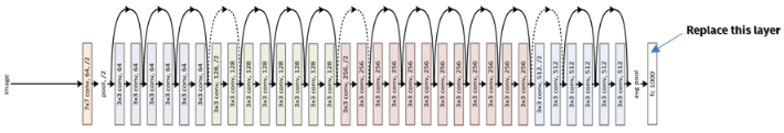
Rather than random initialization of weights in each layer we considered ImageNet initialization for each CNN topology, our DL accuracy have increased substantially when we used ImageNet initialization than random.

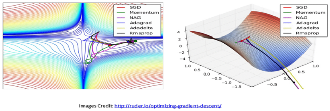
Loss Function and Optimizer:

Cross Entropy loss: Cross-entropy loss, or log loss, measures the performance of a classification model whose output is a probability value between 0 and 1. Cross-entropy loss increases as the predicted probability diverges from the actual label. So predicting a probability of .01 when the actual observation label is 1 would be bad and result in a high loss value. A perfect model would have a log loss of 0
SGD and Nesterov momentum: SGD or stochastic gradient descent is an iterative method for optimizing a differentiable objective function (loss function), it’s stochastic because it takes random samples from the data to do the gradient descent update. Momentum is a moving average of the gradients, it is used to update the weight of the network and it helps accelerate gradients in the right direction. Nesterov is a version of the momentum that is getting popular recently.

4. Case Study: Our Second approach

Critique to first approach: While extracting regions of interest, it requires rewriting code whenever there are changes in product types, circuit board type/chip type (in case of our abstract example), camera setups / directions etc. This is not scalable.

Solution: We built an end-end two step DL architecture. In the first step, instead of a CV approach we used a DL approach to predict the ROI itself. We manually created a labelled dataset with a bounding box tool & we let train a DL architecture to predict the ROI. One downside of this technique is that the labelled dataset has to be explicit and extensive enough to include all product types etc. (circuit board type/chip type in case of our abstract example) for the deep neural network to generalize well on unseen images. Refer the figures below:

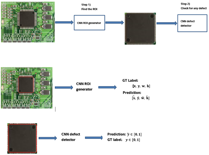
4.1. CNN ROI generator Loss function:

· We initially used a squared distance based loss function as below :

After training a Resnet50 model for 20 epochs we achieved the following validation metric (average missed area and IOU) on the validation set :

Ave. missed area = 8.52 * 10-3

Ave. IOU (intersection over union) = 0.7817

At least, we want to improve the IOU

· We came up with an Area based loss, please refer the figure below to get an idea of how we use basic math to calculate the area of intersection between the ground truth and the predicted label. In the loss function, we want to penalize both the missed and the excess area. Ideally, we would want to penalize the missed area more than the excess area:

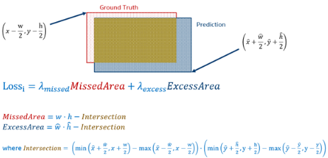
The Loss function above is differentiable so we can do gradient descent optimization on the loss function

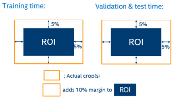
4.2. CNN ROI generator Augmentation: we simply added margins 5% (both left and right) margins during training time and test time on our predicted ROIs:

4.3. CNN ROI generator results: We used Resnet50 (ImageNet initilization) toplogy and SGD + Nesterov momentum optimizer with penalty term “lamda missed” =2 & penalty term “lamda excess” =1 in the area based loss as described above. After training the Resnet50 model for multiple epochs we want to minimize the avg. missed area and maximize the avg. IOU (Best IOU is ‘1’). After training for 20 epochs we achieved the following on the validation set:

Ave. missed area = 3.65 * 10-3

Ave. IOU (intersection over union) = 0.8577

With area based loss and augmentation(described above) we improved our validation metric on missed area and IOU

4.4. Experiments & Benchmarks:

Experiment:

Total # of images: Few thousand images

Data split: 80-to-10-to-10 split, using unique images only

Framework used: PyTorch & Tensorflow / Keras

Weights Initialization: Pre-trained on ImageNet

Optimizer: SGD with learning rate = 0.001, using Nesterov with momentum = 0.9

Loss: Cross entropy

Batch size: 12

Total # of epochs: 24

Image shape: 224x224x3 (except for Inception V3, which requires 299x299x3)

Criterion: Lowest validation loss

Benchmarks

Our benchmarks with both the approaches are pretty comparable, the results with CV+DL (first) approach are little better off than the DL+DL (second) approach. We believe, our DL+DL could be better if we can create an extensive and explicit labelled bounding box dataset.

Following a successful completion of training, an inference solution has to be found to complete the whole end to end solution. We used Intel OpenVino software to optimize inference in different types of hardware besides CPU such as FPGA, Intel Movidius etc.

Inference

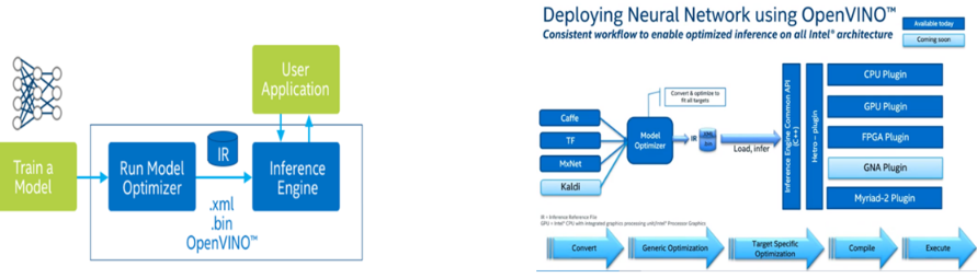
Intel Open Vino: Based on convolution neural networks (CNN), the Intel Open Vino toolkit extends workloads across Intel hardware and maximizes performance:

Enables CNN-based deep learning inference on the edge
Supports heterogeneous execution across computer vision accelerators—CPU, GPU, Intel® Movidius™ Neural Compute Stick, and FPGA—using a common API
Speeds time to market via a library of functions and pre-optimized kernels
Includes optimized calls for OpenCV and OpenVX*

Refer the following figures on Open Vino architecture:

5. Two Step Deployment

5.1. Step one is to convert the pre-trained model into intermediate representations (IRs) using Model Optimizer:

Produce a valid intermediate representation: If this main conversion artifact is not valid, the Inference Engine cannot run. The primary responsibility of the Model optimizer is to produce the two files to form the Intermediate Representation.
Produce an optimized intermediate representation: Pre-trained models contain layers that are important for training, such as the dropout layer. These layers are useless during inference and might increase the inference time. In many cases, these layers can be automatically removed from the resulting Intermediate Representation. However, if a group of layers can be represented as one mathematical operation, and thus as a single layer, the Model Optimizer recognizes such patterns and replaces these layers with one. The result is an Intermediate Representation that has fewer layers than the original model. This decreases the inference time.

The IR is a pair of files that describe the whole model:

xml: Describes the network topology
bin: Contains the weights and biases binary data

5.2. Step two is to use the Inference Engine to read, load, and infer the IR files, using a common API across the CPU, GPU, or VPU hardware

Open Vino documentation: https://software.intel.com/en-us/inference-trained-models-with-inte…

5.3. Inference Benchmarks on sample Image:

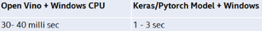
It is clear that optimizing with software stack is critical to reduce the inference time. We saw 30X to 100X improvement in latency time using OpenVino software optimization. In addition, besides Intel CPU we also experimented with other Intel hardware accelerators such as Intel Movidius and FPGA.

6. Visualizing CNN with Heat Maps

Often deep neural networks are criticized for low interpretability and most deep learning solutions stop at the point when the classification of the labels are done. We wanted to interpret our results, why the CNN architecture labelled an image as good or bad (binary classification for our case study), which area in the image the CNN is focusing most.

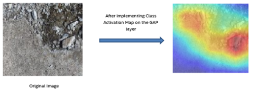
Based on this research in MIT https://arxiv.org/pdf/1512.04150.pdf , a class activation map in combination with the global max pooling layer has been proposed to localize class specific image regions.

Global average pooling usually acts as a regularizer, preventing overfitting during training. It is established in this research that the advantages of global average pooling layer extend beyond simply acting as a regularizer – little tweaking, the network can retain its remarkable localization ability until the final layer. This tweaking allows identifying easily the discriminative image regions in a single forward pass for a wide variety of tasks, even those that the network was not originally trained for.

Following is a heat map interpretation using this technique on the “crack on a plain surface” image using Resnet-50 architecture trained on ImageNet. As we can see, the heat map focusses on the crack area below although the architecture is not trained on such images –

7. Summary & Conclusion

With deep learning based computer vision we achieved human level accuracy and better with both of our approaches – CV+DL and DL+DL (discussed earlier in this blog). Our solution is unique – we not only used deep learning for classification but for interpreting the defect area with heat maps on the image itself.

Human factor cannot be completely dissociated but we can substantial reduce human intervention. An optimal model is always a fine tune between FPR (false positive rate) & FNR (false negative rate) or Precision vs Recall. For our use case, we successfully automated defect detection with a model optimized for low FNR (High Recall). We substantially reduced the human review rate. With our case study we proved that we can automate material inspection with deep learning & reduce human review rate.

References: