
Picture by By Tatiana Shepeleva/shutterstock.com
One of the most challenging problems in modern theoretical physics is the so-called many-body problem. Typical many-body systems are composed of a large number of strongly interacting particles. Few such systems are amenable to exact mathematical treatment and numerical techniques are needed to make progress. However, since the resources required to specify a generic many-body quantum state depend exponentially on the number of particles in the system (more precisely, on the number of degrees of freedom), even today’s best supercomputers lack sufficient power to exactly encode such states (they can handle only relatively small systems, with less than ~45 particles).
As we shall see, recent applications of machine learning techniques (artificial neural networks in particular) have been shown to provide highly efficient representations of such complex states, making their overwhelming complexity computationally tractable.
In this article, I will discuss how to apply (a type of) artificial neural network to represent quantum states of many particles. The article will be divided into three parts:
- A bird’s-eye view of fundamental quantum mechanical concepts.
- A brief description of machine learning concepts with a particular focus on a type of artificial neural network known as Restricted Boltzmann Machine (RBM)
- An explanation of how one can use RBMs to represent many-particle quantum states.
A Preamble
There is a fascinating story recounted by one of Albert Einstein’s scientific collaborators, the Polish physicist Leopold Infeld, in his autobiography.
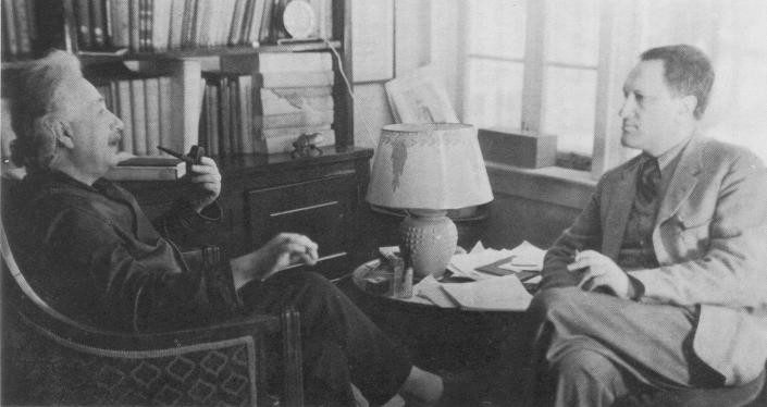
Einstein and Infeld in Einstein’s home (source).
According to Infeld, after the two physicists spent several months performing long and grueling calculations, Einstein would make the following remark:
“God [Nature] does not care about our mathematical difficulties. He integrates empirically.”
— Einstein (1942).
What Einstein meant was that, while humans must resort to complex calculations and symbolic reasoning to solve complicated physics problems, Nature does not need to.
Quick Note: Einstein used the term “integrate” here because many physical theories are formulated using equations called “differential equations” and to find solutions of such equations one must apply the process of “integration”.
The Many-Body Problem
As noted in the introduction, a notoriously difficult problem in theoretical physics is the many-body problem. This problem has been investigated for a very long time in both classical systems (physical systems based on Newton’s three laws of motion and its refinements) and quantum systems (systems based obeying quantum mechanical laws).
The first (classical) many-body problem to be extensively studied was the 3-body problem involving the Earth, the Moon, and the Sun.
A simple orbit of a 3-body system with equal masses.
One of the first scientists to attack this many-body problem was none other than Issac Newton in his masterpiece, the Principia Mathematica:
“Each time a planet revolves it traces a fresh orbit […] and each orbit is dependent upon the combined motions of all the planets, not to mention their actions upon each other […]. Unless I am much mistaken, it would exceed the force of human wit to consider so many causes of motion at the same time, and to define the motions by exact laws which would allow of an easy calculation.”
— Isaac Newton (1687)
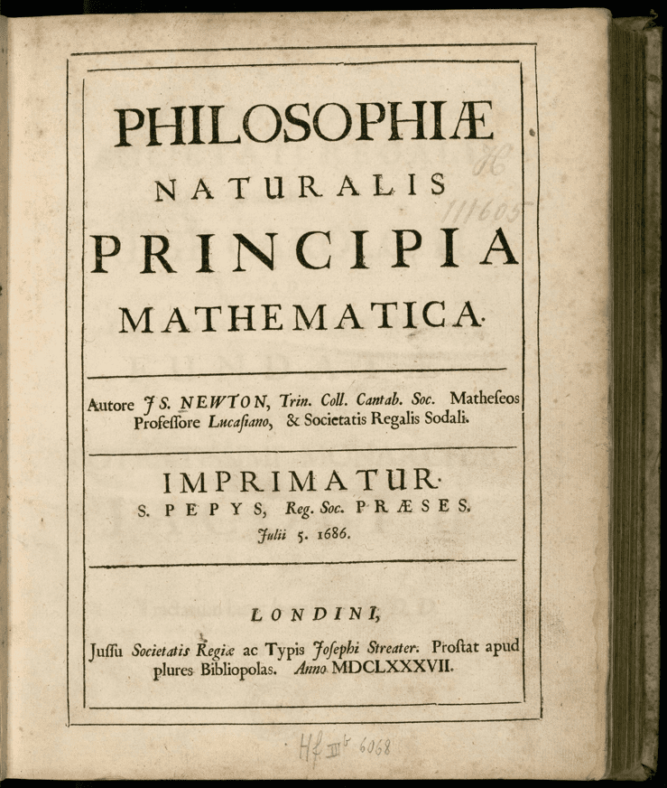
Newton’s Principia Mathematica, arguably the most important scientific book in history.
Since essentially all relevant physical systems are composed by a collection of interacting particles, the many-body problem is extremely important.
A Poor Man’s Definition
One can define the problem as “the study of the effects of interactions between bodies on the behavior of a many-body system ”.
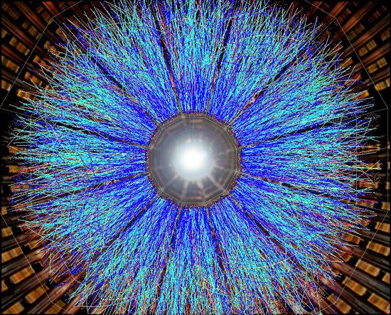
Collisions of gold ions generate a quark-gluon plasma, a typical many-body system.
The meaning of “many” in this context can be anywhere from three to infinity. In a recent paper, my colleagues and I showed that the signatures of quantum many-body behavior can be found already for N=5 spin excitations (figure below).
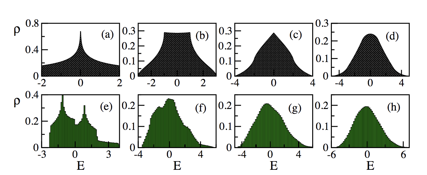
The density of states of a type of spin system (XX model). As the number of spin excitations increases from 2 to 5, a Gaussian distribution (typical of many-body systems with 2-body couplings) is approached.
In the present article, I will focus on the quantum many-body problem which has been my main topic of research since 2013.
Quantum Many-Body Systems
The complexity of quantum many-body systems was identified by physicists already in the 1930s. Around that time, the great physicist Paul Dirac envisioned two major problems in quantum mechanics.
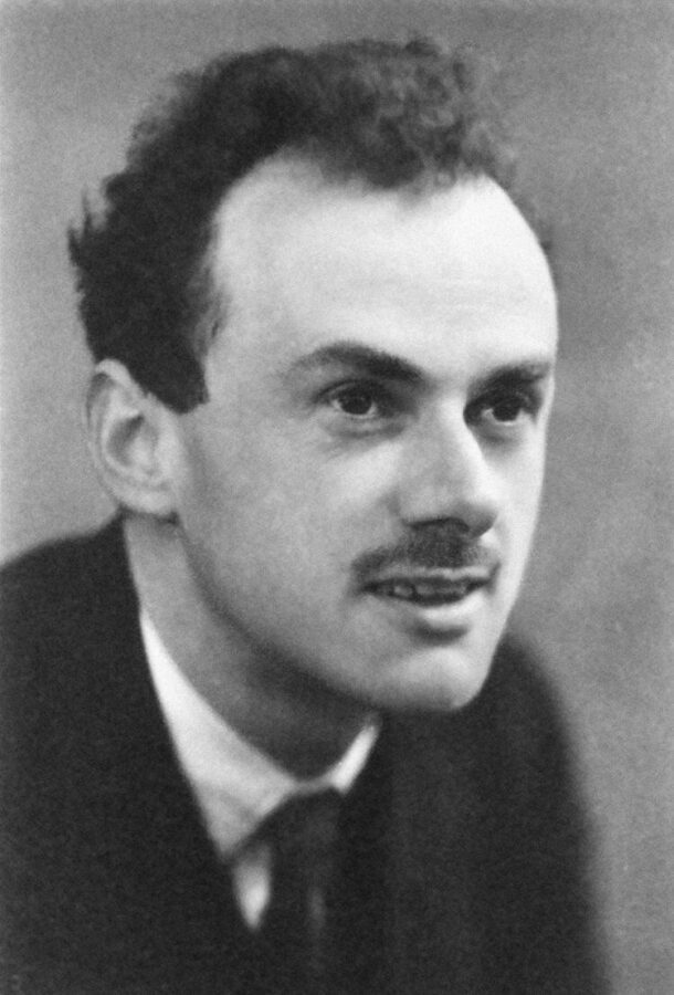
The English physicist Paul Dirac.
The first, according to him, was “in connection with the exact fitting in of the theory with relativity ideas”. The second was that “the exact application of these [quantum] laws leads to equations much too complicated to be soluble”. The second problem was precisely the quantum many-body problem.
Luckily, the quantum states of many physical systems can be described using much less information than the maximum capacity of their Hilbert spaces. This fact is exploited by several numerical techniques including the well-known Quantum Monte Carlo (QMC) method.
Quantum Wave Functions
Simply put, a quantum wave function describes mathematically the state of a quantum system. The first quantum system to receive an exact mathematical treatment was the hydrogen atom.
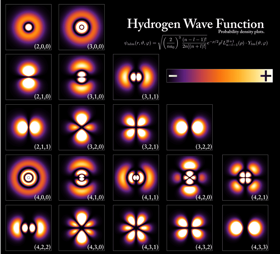
The probability of finding the electron in a hydrogen atom (represented by the brightness).
In general, a quantum state is represented by a complex probability amplitude Ψ(S), where the argument S contains all the information about the system’s state. For example, in a spin-1/2 chain:
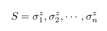
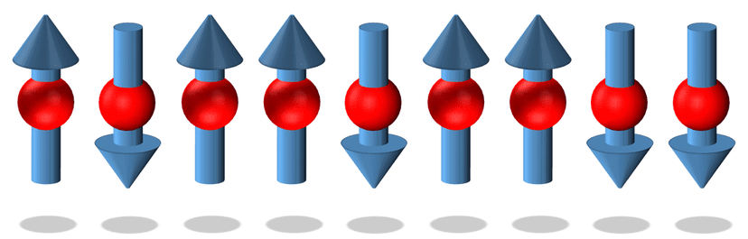
A 1D spin chain: each particle has a value for σ in the z-axis.
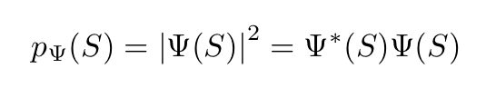
From Ψ(S), probabilities associated with measurements made on the system can be derived. For example, the square modulus of Ψ(S), a positive real number, gives the probability distribution associated with Ψ(S):
The Hamiltonian Operator
The properties of a quantum system are encapsulated by the system’s Hamiltonian operator H. The latter is the sum of two terms:
- The kinetic energy of all particles in the system and it is associated with their motion
- The potential energy of all particles in the system, associated with the position of the particles with respect to other particles.
The allowed energy levels of a quantum system (its energy spectrum) can be obtained by solving the so-called Schrodinger equation, a partial differential equation that describes the behavior of quantum mechanical systems.
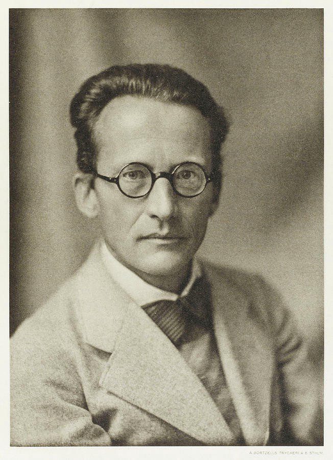
The Austrian physicist Erwin Schrodinger, one of the fathers of quantum mechanics .
The time-independent version of the Schrödinger equation is given by the following eigenvalue system:
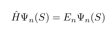
The eigenvalues and the corresponding eigenstates are
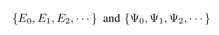
The lowest energy corresponds to the so-called “ground state” of the system.
A Simple Example
For concreteness, let us consider the following example: the quantum harmonic oscillator. The QHO is the quantum-mechanical counterpart of the classical harmonic oscillator (see the figure below), which is a system that experiences a force when displaced from its initial that restores it to its equilibrium position.
A mass-spring harmonic oscillator
The animation below compares the classical and quantum conceptions of a simple harmonic oscillator.
Wave function describing a quantum harmonic oscillator (Wiki).
While a simple oscillating mass in a well-defined trajectory represents the classical system (blocks A and B in the figure above), the corresponding quantum system is represented by a complex wave function. In each block (from C onwards) there are two curves: the blue one is the real part of Ψ, and the red one is the imaginary part.
Bird’s-eye View of Quantum Spin Systems
In quantum mechanics, spin can be roughly understood as an “intrinsic form of angular momentum” that is carried by particles and nuclei. Though it is intuitive to think of spin as a rotation of a particle around its own axis this picture is not quite correct since then the particle would rotate at a faster than light speed which would violate fundamental physical principles. If fact spins are quantum mechanical objects without classical counterpart.

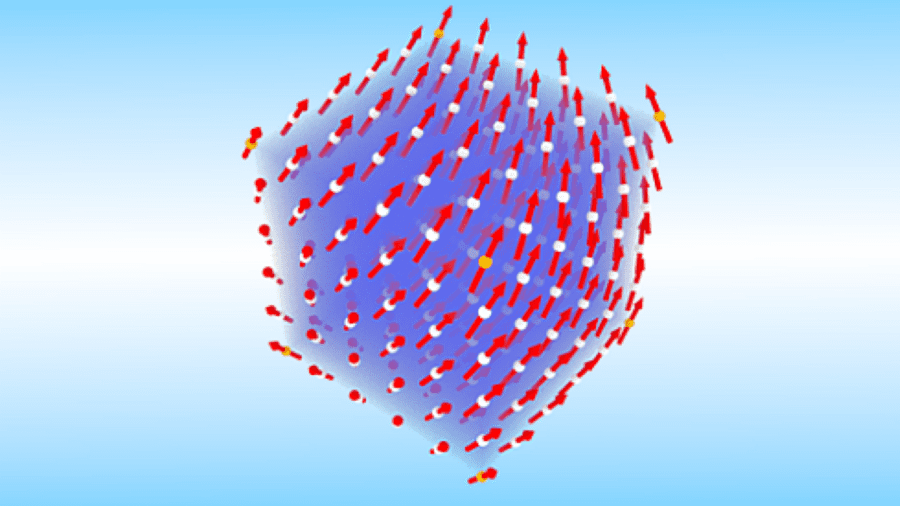
Example of a many-body system: a spin impurity propagating through a chain of atoms
Quantum spin systems are closely associated with the phenomena of magnetism. Magnets are made of atoms, which are often small magnets. When these atomic magnets become parallelly oriented they give origin to the macroscopic effect we are familiar with.
Magnetic materials often display spin waves, propagating disturbances in the magnetic order.
I will now provide a quick summary of the basic components of machine learning algorithms in a way that will be helpful for the reader to understand their connections with quantum systems.
Machine Learning = Machine + Learning
Machine learning approaches have two basic components (Carleo, 2017):
- The machine, which could be e.g. an artificial neural network Ψ with parameters
- The learning of the parameters W, performed using e.g. stochastic optimization algorithms.
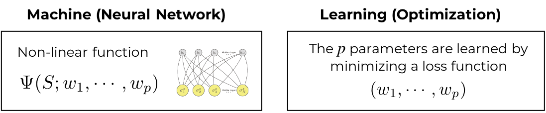
The two components of machine learning.
Neural networks
Artificial neural networks are usually non-linear multi-dimensional nested functions. Their internal workings are only heuristically understood and investigating their structure does not generate insights regarding the function being it approximates.
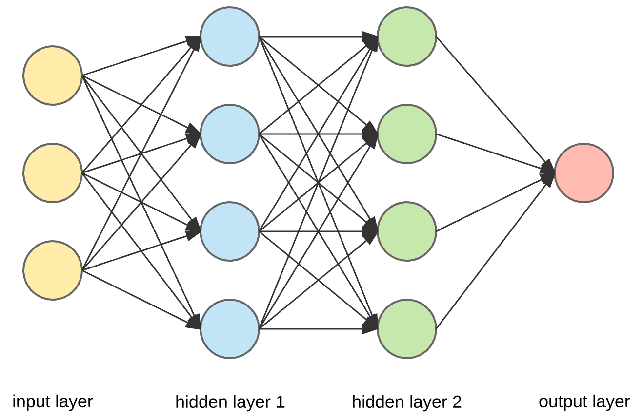
Simple artificial neural network with two hidden layers.
Due to the absence of a clear-cut connection between the network parameters and the mathematical function which is being approximated, ANNs are often referred to as “black boxes”.
What are Restricted Boltzmann Machines?
Restricted Boltzmann Machines are generative stochastic neural networks. They have many applications including:
- Collaborative filtering
- Dimensionality reduction
- Classification
- Regression
- Feature learning
- Topic modeling
RBMs belong to a class of models known as Energy-based Models. They are different from other (more popular) neural networks which estimate a value based on inputs while RBMs estimate probability densities of the inputs (they estimate many points instead of a single value).
RBMs have the following properties:
- They are shallow networks, with only two layers (the input/visible layer and a hidden layer)
- Their hidden units h and visible (input) units v are usually binary-valued
- There is a weight matrix W associated with the connections between hidden and visible units
- There are two bias terms, one for input units denoted by a and one for hidden units denoted by b
- Each configuration has an associated energy functional E(v,h) which is minimized during training
- They have no output layer
- There are no intra-layer connections (this is the “restriction”). For a given set of visible unit activations, the hidden unit activations are mutually independent (the converse also holds). This property facilitates the analysis tremendously.
The energy functional to be minimized is given by:
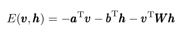
Eq.1: Energy functional minimized by RBMs.
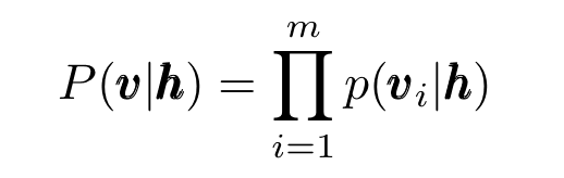
The joint probability distribution of both visible and hidden units reads:
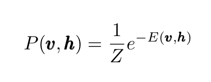
Eq.2: Total probability distribution.
where the normalization constant Z is called the partition function. Tracing out the hidden units, we obtain the marginal probability of a visible (input) vector:
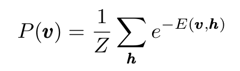
Eq.3: Input units marginal probability distribution,
Since, as noted before, hidden (visible) unit activations are mutually independent given the visible (hidden) unit activations one can write:
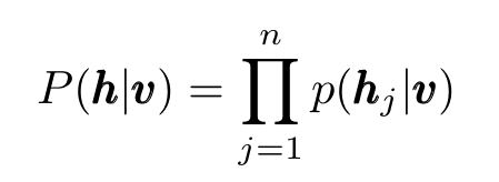
Eq.4: Conditional probabilities becomes products due to mutual independence.
and also:
Eq. 5: Same as Eq.4.
Finally, the activation probabilities read:
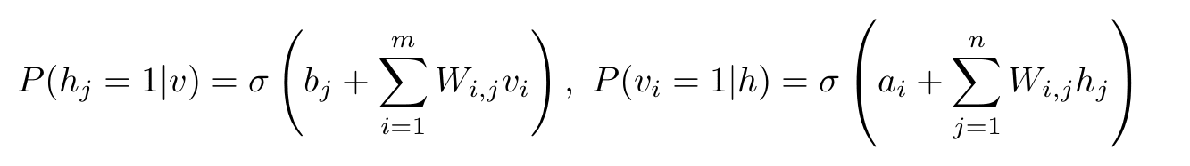
Eq.6: Activation probabilities.
where σ is the sigmoid function.
The training steps are the following:
- We begin by setting the visible units states to a training vector.
- The states of the hidden units are then calculated using the expression on the left of Equation 6.
- After the states are chosen for the hidden units, one performs the so-called “reconstruction”, setting each visible unit to 1 according to the expression on the right of Equation 6.
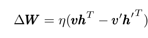
- The weight changes by (the primed variables are the reconstructions):
How RBMs process inputs, a simple example
The following analysis is heavily based on this excellent tutorial. The three figures below show how a RBM processes inputs.
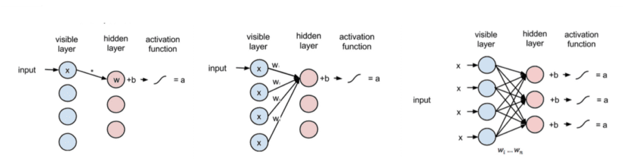
A simple RBM processing inputs.
- At node 1 of the hidden layer, the input x is multiplied by the weight w, a bias b is added, and the result is fed into the activation giving origin to an output a (see the leftmost diagram).
- In the central diagram, all inputs are combined at the hidden node 1 and each input x is multiplied by its corresponding w. The products are then summed, a bias b is added, and the end result is passed into an activation function producing the full output a from the hidden node 1
- In the third diagram, inputs x are passed to all nodes in the hidden layer. At each hidden node, x is multiplied by its corresponding weight w. Individual hidden nodes receive products of all inputs x with their individual weights w. The bias b is then added to each sum, and the results are passed through activation functions generating outputs for all hidden nodes.
How RBMs learn to reconstruct data
RBMs perform an unsupervised process called “reconstruction”. They learn to reconstruct the data performing a long succession of passes (forward and backward ones) between its two layers. In the backward pass, as shown in the diagram below, the activation functions of the nodes in the hidden layer become the new inputs.
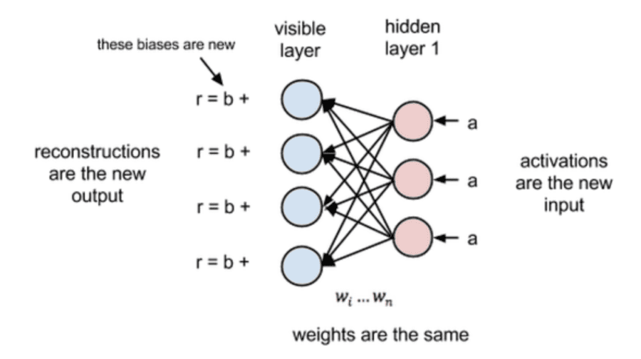
The product of these inputs and the respective weights are summed and the new biases b from the visible layer are added at each input node. The new output from such operations is called “reconstruction” because it is an approximation of the original input.
Naturally, the reconstructions and the original inputs are very different at first (since the values of w are randomly initialized). However, as the error is repeatedly backpropagated against the ws, it is gradually minimized.
We see therefore that:
- The RBM uses, on the forward pass, inputs to make predictions about the activations of the nodes and estimate the probability distribution of the output a conditional on the weighted inputs x
- On the backward pass, the RBM tries to estimate the probability distribution of the inputs x conditional on the activations a
Joining both conditional distributions, the joint probability distribution of x and a is obtained i.e. the RBM learns how to approximate the original data (the structure of the input).
How to connect machine learning and quantum systems?
In a recent article published in Science magazine, it was proposed that one can treat the quantum wave function Ψ(S) of a quantum many-body system as a black-box and then approximate it using an RBM. The RBM is trained to represent Ψ(S) via the optimization of its parameters.
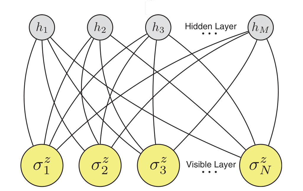
RBM used by Carleo and Troyer (2017) that encodes a spin many-body quantum state.
The question is how to reformulate the (time-independent) Schrodinger equation, which is an eigenvalue problem, as a machine learning problem.
Variational Methods
As it turns out, the answer has been known for quite some time, and it is based on the so-called variation method , an alternative formulation of the wave equation that can be used to obtain the energies of a quantum system. Using this method we can write the optimization problem as follows:

where E[Ψ] is a functional that depends on the eigenstates and Hamiltonian. Solving this optimization problem we obtain both the ground state energy and its corresponding ground state.
Quantum States and Restricted Boltzmann Machines
In Carleo and Troyer (2017), RBMs are used to represent a quantum state Ψ(S). They generalize RBMs to allow for complex network parameters.
It is easy to show that the energy functional can be written as
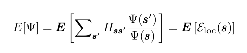
where the argument of the expectation value after the last equal sign is the local energy. The neural network is then trained using the method of Stochastic Reconfiguation (SR). The corresponding optimization iteration reads:
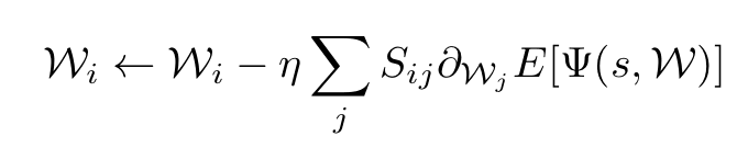
The gradient descent update protocol.
where η is the learning rate and S is the stochastic reconfiguration matrix which depends on the eigenstates and its logarithmic derivatives.
Carleo and Troyer (2017)were interested specifically in quantum systems of spin 1/2 and they write the quantum state as follows:

In this expression the W argument of Ψ is the set of parameters:

where the components on a and b are real but W can be complex. The absence of intralayer interactions, typical of the RBMs architecture allows hidden variables to be summer over (or traced out), considerably simplifying the expression above to:

To train the quantum wave functions one follows a similar procedure as described above for RBMs.
Impressive Accuracy
The figure below shows the negligible relative error of the NQS ground-state energy estimation. Each plot corresponds to a test case which is a system with known exact solutions. The horizontal axis is the hidden-unit density i.e. the ratio between the number of hidden and visible units. Notice that even with relatively few hidden units, the accuracy of the model is already extremely impressive (one part per million error!)
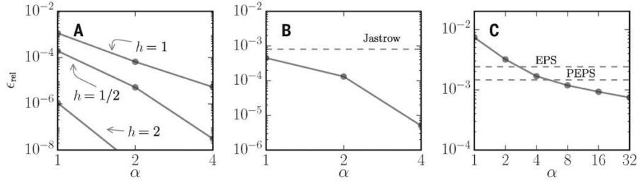
The error of the model ground-state energy relative to the exact value in three tests cases.
Conclusion
In this brief article, we saw that Restricted Boltzmann Machines (RBMs), a simple type of artificial neural network, can be used to compute with extremely high accuracy the ground-state energy of quantum systems of many particles.
Thanks for reading!
As always, constructive criticism and feedback are welcome!
This article was originally published on here.