
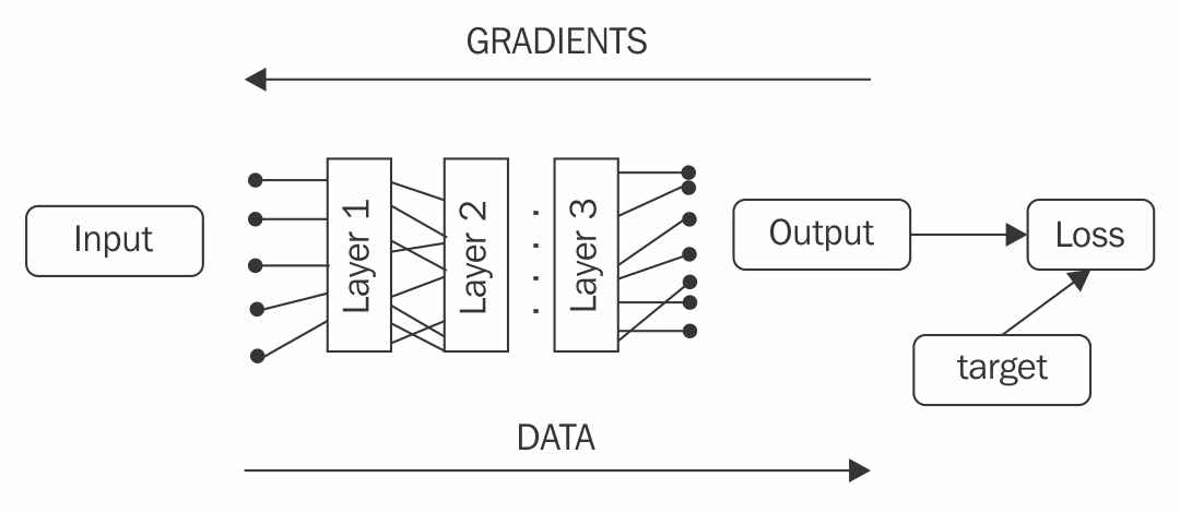
In this article by Maxim Lapan, the author of Deep Reinforcement Learning Hands-On,we are going to discuss about gradients in PyTorch.
Gradients support in tensors is one of the major changes in PyTorch 0.4.0. In previous versions, graph tracking and gradients accumulation were done in a separate, very thin class Variable, which worked as a wrapper around the tensor and automatically performed saving of the history of computations in order to be able to backpropagate. Now gradients are a built-in tensor property, which makes the API much cleaner.
The automatic computation of Gradients
Gradient was originally implemented in the Caffe toolkit and then became the de-facto standard in DL libraries. Computing gradients manually was extremely painful to implement and debug, even for the simplest neural network (NN). You had to calculate derivatives for all your functions, apply the chain rule, and then implement the result of the calculations, praying that everything was done right. This could be a very useful exercise for understanding the nuts and bolts of DL, but it’s not something that you wanted to repeat over and over again by experimenting with different NN architectures.
Luckily, those days have gone now, much like programming your hardware using a soldering iron and vacuum tubes! Now defining an NN of hundreds of layers requires nothing more than assembling it from predefined building blocks or, in the extreme case of you doing something fancy, defining the transformation expression manually. All gradients will be carefully calculated for you, backpropagated, and applied to the network. To be able to achieve this, you need to define your network architecture in terms of the DL library used, which can be different in details, but in general, must be the same: you define the order in which your network will transform inputs to outputs.
- Static graph: In this method, you need to define your calculations in advance and it won’t be possible to change them later. The graph gets processed and optimized by the DL library before any computation can be made. This model is implemented in TensorFlow, Theano, and many other DL toolkits.
- Dynamic graph: You don’t need to define your graph in advance exactly as it will be executed. You just execute operations that you want to use for data transformation on your actual data. During this, the library records the order of operations performed, and when you ask it to calculate gradients, it unrolls its history of operations, accumulating the gradients of network parameters. This method is also called notebook gradients and is implemented in PyTorch, Chainer, and some others.
Both methods have their strengths and weaknesses. For example, static graph is usually faster, as all computations can be moved to the GPU, minimizing the data transfer overhead. Additionally, in static graph, the library has much more freedom in optimizing the order that computations are performed in or even removing parts of the graph. On the other hand, dynamic graph has a higher computation overhead, but gives a developer much more freedom. For example, they can say, “For this piece of data, I can apply this network two times, and for this piece of data, I’ll use a completely different model with gradients clipped by the batch mean.” Another very appealing strength of the dynamic graph model is that it allows you to express your transformation more naturally, in a more “Pythonic” way. In the end, it’s just a Python library with bunch of functions, so just call them and let the library do the magic.
Tensors and gradients
PyTorch tensors have a built-in gradient calculation and tracking machinery, so all you need to do is to convert the data into tensors and perform computations using the tensor’s methods and functions provided by torch. Of course, if you need to access underlying low-level details, you always can, but most of the time, PyTorch does what you’re expecting.
There are several attributes related to gradients that every tensor has:
- grad: A property which holds a tensor of the same shape containing computed gradients.
- is_leaf: True, if this tensor was constructed by the user and False, if the object is a result of function transformation.
- requires_grad: True if this tensor requires gradients to be calculated. This property is inherited from leaf tensors, which get this value from the tensor construction step (zeros() or torch.tensor() and so on). By default, the constructor has requires_grad=False, so if you want gradients to be calculated for your tensor, then you need to explicitly say so.
To make all of this gradient-leaf machinery clearer, let’s consider this session:
>>> v1 = torch.tensor([1.0, 1.0], requires_grad=True)
>>> v2 = torch.tensor([2.0, 2.0])
In the preceding code, we created two tensors. The first requires gradients to be calculated and the second doesn’t:
>>> v_sum = v1 + v2
>>> v_res = (v_sum*2).sum()
>>> v_res
tensor(12.)
So now we’ve added both vectors element-wise (which is vector [3, 3]), doubled every element, and summed them together. The result is a zero-dimension tensor with the value 12. Okay, so this is simple math so far. Now let’s look at the underlying graph that our expressions created:
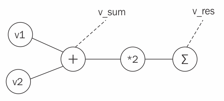
If we check the attributes of our tensors, then we find that v1 and v2 are the only leaf nodes and every variable except v2 requires gradients to be calculated:
>>> v1.is_leaf, v2.is_leaf
(True, True)
>>> v_sum.is_leaf, v_res.is_leaf
(False, False)
>>> v1.requires_grad
True
>>> v2.requires_grad
False
>>> v_sum.requires_grad
True
>>> v_res.requires_grad
True
Now, let’s tell PyTorch to calculate the gradients of our graph:
>>> v_res.backward()
>>> v1.grad
tensor([ 2., 2.])
By calling the backward function, we asked PyTorch to calculate the numerical derivative of the v_res variable, with respect to any variable that our graph has. In other words, what influence do small changes to the v_res variable have on the rest of the graph? In our particular example, the value of 2 in v1’s gradients means that by increasing every element of v1 by one, the resulting value of v_res will grow by two.
As mentioned, PyTorch calculates gradients only for leaf tensors with requires_grad=True. Indeed, if we try to check the gradients of v2 we get nothing:
>>> v2.grad
The reason for that is efficiency in terms of computations and memory: in real life, our network can have millions of optimized parameters, with hundreds of intermediate operations performed on them. During gradient descent optimization, we’re not interested in gradients in any intermediate matrix multiplication; the only thing we need to be able to tune the model is gradients of loss with respect to model parameters (weights). Of course, if you want to calculate the gradients of input data (it could be useful if you want to generate some adversarial examples to fool the existing NN or adjust pretrained word embeddings), then you can easily do so, by passing requires_grad=True on tensor creation.
You enjoyed an excerpt from Packt Publishing’s latest book, Deep Reinforcement Learning Hands-On written by Maxim Lapan. If you are a Deep Learning enthusiast, this is the book that you will need to solve complex real-world problems using Deep Learning.