
Bayesian Machine Learning (part -7)
Expectation-Maximization : A solved Example
I have covered the theoretical part of EM algorithm in my previous posts. For reference below are the links:
In the previous posts I have explained the complete derivation of EM algorithm, in this post we take a very simple example and see what all we actually need to remember to apply an EM algorithm on a clustering problem.
So let’s start !!!
Problem Statement
Let us first define our problem statements:
Consider a following type of distribution as shown in the below image :
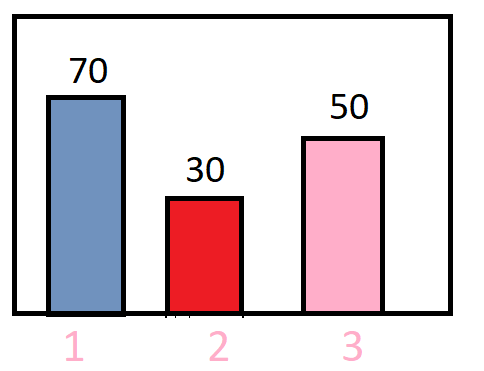
In the above distribution random variable takes 3 values {1,2,3} with frequency {70,30,50} respectively. Our objective is to design a clustering model on the top of it.
Key features about the data:
- The data is discrete in nature
- We can consider the above data as a mixture of 2 probabilistic
- distribution functions
So now our objective is to find the parameters of the defined Pdfs. So let us first define our probability density functions as follows:
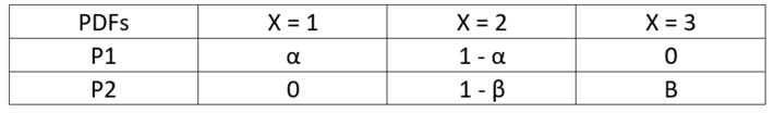
The above expression states that for PDF p1: random variable takes values {1,2,3} with probability { α , 1- α ,0 } respectively and similarly for PDF p2 : random variable takes values {1,2,3} with probability {0, 1 – β , β} respectively.
So now to be more precise we want to compute the exact values of α and β.
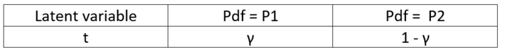
Introduction of Latent Variable in the Scene
Let us say as we need to apply the EM algorithm we need a latent Variable !!!
We consider the concept of latent variable in the case when we are unable to explain the behavior of the observed variable. Latent variable are used to define the behavior of observed variable. In our case of clustering in the above problem, we consider a latent variable t which defines which observed data point comes from which cluster or pdf. function. In other words, which distribution is how much probable.
So, let us define the distribution of our latent variable t.
So now to be more precise, we need to compute the values of γ, α and β.
So, lets start !!
Prior Setting
Let us first consider a prior value for all our variables
γ = α = β = 0.5
now the above equation states that:
P (X = 1 | t = P1) = 0.5
P (X = 2 | t = P1) = 0.5
P (X = 3 | t = P1) = 0
P (X = 1 | t = P2) = 0
P (X = 1 | t = P2) = 0.5
P (X = 1 | t = P2) = 0.5
P (t = P1) = 0.5
P (t = P2) = 0.5
E-Step
To solve the E step we need to focus on the equation shown below:
q(t=c) = P(t=c | Xi , θ)
for i ranging for all the given data points.
Here q is the distribution from the lower bound after we use the Jensen’s inequality.(refer part 5)
So, let us compute the q(t=c) for all the given data points in our problem.
P(t=c | Xi ) = P(Xi | t = c)*P(t=c) / summation on c(P(Xi | t = c)*P(t=c))
P(t=1 | X =1 ) = (α * γ) / (α * γ + 0) = 1
P(t=1 | X =2 ) = ((1 – α) * γ) / ((1-α) * γ + (1- β)*(1- γ)) = 0.5
P(t=1 | X =3 ) = (0 * γ) / (0 * γ + (β)*(1- γ)) = 0
P(t=2 | X =1 ) = (0 * (1-γ)) / (0 * (1-γ)) + (α * γ)) = 0
P(t=2 | X =2 ) = (1- β)*(1- γ) / ((1- β)*(1- γ) + (1-α) * γ) = 0.5
P(t=2 | X =3 ) = (β)*(1- γ) / (β)*(1- γ) + 0 = 1
Wasn’t it simple !!!
Let see M step
M Step
In the M step we need to differentiate the below equation w.r.t γ ,α ,β and use the previously calculated values in E Step as constants. So the equation is :
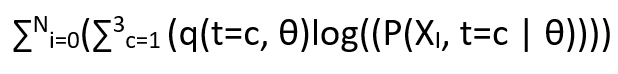
We can ignore θ in the above representation for this problem as it is simple and disrete in nature with direct probabilities for 3 values.
So, now the new representation is as :
Likelihood lower bound differential part = 
To remember the above expression is simple:
Summation on datapoint(summation on q the values we computed in E step(log of joint distribution over Xi and t))
So, let us expand our equation, we will differentiate to compute our parameters

Solving the above equation by differentiating the equation 3 times, each time w.r.t 1 paramter and keeping the other 2 as constant we end up to the following result:
γ = (85/150), α = (70/85) , β = (50/65)
Now you can check the calculation yourself, these were my hand performed results 🙂
Now we can again put the above computed paramter values in the E step for computation of the posterior and then again perform M step.(most probably the values won;t change for the above problem)
We do the above iterations until our parameters values stop updating.
And this is how we perform our EM algorithm !!!
Once we know the values of our paramters, we know our probability density function of P1 and P2. Now for any new value taken by our random variable X, we can specifically say from which cluster of pdf function it belongs and with what probability.
Thanks for reading !!!