
This article was written by Giuseppe Bonaccorso.
Stochastic Gradient Descent (SGD) is a very powerful technique, currently employed to optimize all deep learning models. However, the vanilla algorithm has many limitations, in particular when the system is ill-conditioned and could never find the global minimum. In this post, we’re going to analyze how it works and the most important variations that can speed up the convergence in deep models.
First of all, it’s necessary to standardize the naming. In some books, the expression “Stochastic Gradient Descent” refers to an algorithm which operates on a batch size equal to 1, while “Mini-batch Gradient Descent” is adopted when the batch size is greater than 1. In this context, we assume that Stochastic Gradient Descent operates on batch sizes equal or greater than 1.
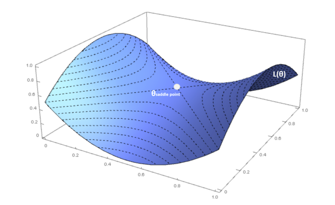
In a standard optimization problem, without particular requirements, the algorithm converges in a limited number of iterations. Unfortunately, the reality is a little bit different, in particular in deep models, where the number of parameters is in the order of ten or one hundred million. When the system is relatively shallow, it’s easier to find local minima where the training process can stop, while in deeper models, the probability of a local minimum becomes smaller and, instead, saddle points become more and more likely.
If the Hessian matrix is (m x m) where m is the number of parameters, the second condition is equivalent to say that all m eigenvalues must be non-negative (or that all principal minors composed with the first n rows and n columns must be non-negative).
From a probabilistic viewpoint, P(H positive semi-def.) → 0 when m → ∞, therefore local minima are rare in deep models (this doesn’t mean that local minima are impossible, but their relative weight is lower and lower in deeper models). If the Hessian matrix has both positive and negative eigenvalues (and the gradient is null), the Hessian is said to be indefinite and the point is called saddle point. In this case, the point is maximum considering an orthogonal projection and a minimum for another one.
Now we’re going to discuss some common methods to improve the performance of a vanilla Stochastic Gradient Descent algorithm.
Gradient Perturbation
A very simple approach to the problem of plateaus is adding a small noisy term (Gaussian noise) to the gradient.
The variance should be carefully chosen (for example, it could decay exponentially during the epochs). However, this method can be a very simple and effective solution to allow a movement even in regions where the gradient is close to zero.
Momentum and Nesterov Momentum
The previous approach was quite simple and in many cases, it can difficult to implement. A more robust solution is provided by introducing an exponentially weighted moving average for the gradients. The idea is very intuitive: instead of considering only the current gradient, we can attach part of its history to the correction factor, so to avoid an abrupt change when the surface becomes flat.
RMSProp
This algorithm, proposed by G. Hinton, is based on the idea to adapt the correction factor for each parameter, so to increase the effect on slowly-changing parameters and reduce it when their change magnitude is very large. This approach can dramatically improve the performance of a deep network, but it’s a little bit more expensive than Momentum because we need to compute a speed term for each parameter.
To read the whole article, with formulas and illustrations, click here.