
Abstract
In this study, we predict the outcome of the football matches in the FIFA World Cup 2018 to be held in Russia this summer. We do this using classification models over a dataset of historic football results that includes attributes from the playing teams by rating them in attack, midfield, defence, aggression, pressure, chance creation and building ability. This last training data was a result of merging international matches results with AE games ratings of the teams considering the timeline of the matches with their respective statistics. Final predictions show the four countries with the most chances of getting to the semifinals as France, Brazil, Spain and Germany while giving Spain as the winner.
Dataset
The objective of this study is to build a predictive model that will allow us to make good predictions for the coming World Cup 2018 so we looked for dataset with historic data for match results, for this purpose we chose a dataset from Kaggle with data of almost 40,000 international matches played between 1872 and 2018. This dataset however did not have attributes related to the teams playing, so we looked for information about historic data of teams stats and for that we found a website called sofifa that updated constantly the stats the EA videogame use about them, it hold information for the last 10 years with biannual updates to the first years and more constant updated for the last few years.
The following tables show the variables included in each dataset we originally used for this study
International matches between 1872 and 2018
- home_team: Team playing as home
- away_team: Team playing as visitor
- home_team_goals: Goals scored by the home_team
- away_team_goals: Goals scored by the away_team
- tournament: Tournament organizing the match
- date: Date of the match
- country: Country were the match took place
- neutral: True if the match was not played in the home country
Team ratings from Sofifa.com since 2010
- date: Date for the stats
- team: Name of the team
- Overall: Overall rating of the team (1-100)
- Attack: Attack rating of the team (1-100)
- midfield: Midfield rating of the team (1-100)
- defense: Defense rating of the team (1-100)
- bu_speed: Building speed rating of the team (1-100)
- bu_passing: Building passing rating of the team (1-100)
- bu_shooting: Building shooting rating of the team (1-100)
- bu_position: Building position (Organized or Freeform)
- cc_crossing: Chance creation crossing rating of the team (1-100)
- cc_passing: Chance creation passing rating of the team (1-100)
- cc_shooting: Chance creation shooting rating of the team (1-100)
- cc_position:Chance creation position (Organized or Freeform)
- aggression: Aggression rating of the team (1-100)
- pressure: Pressure rating of the team (1-100)
- age: Average age of the team players
Preprocessing
For the preprocessing part of our project, we needed to create a final dataset with stats for both teams participating in each match, so the first thing to do was to merge the match file with the stats file twice, one for each team. The tool we used for this task was R and the first problem we encountered was the discrepancy between the names, like for example USA and United States, so we had to correct that by changing some of the countries names in the sofifa dataset to match to the main one; after this, we used the sqldf package which allowed us to use SQL language to manipulate data frames in R; the condition for the merge was that each team should have the stats for the latest date available in the sofifa file considering the date of the match.
Once the merge was performed, we only wanted to keep rows with complete data. There are many countries that don’t appear in the sofifa web site but also there was only complete information for them available since 2010. So by dropping rows with missing values, we ended up with 1,183 observations of international matches since 2010 where the stats for the two teams were available.
Since home and away is a condition that doesn’t apply in the world cup, we decided to rearrange the teams based on their overall rank and instead of home and away team, we rearranged the data and created strong and weak team which includes rearranging all of their stats as well. We also created new fields to be used as predictors which are the differences for each stat between the strong and the weak team.
Finally we needed a dependant variable for our analysis so we created the variable win. First we created three classes for this win labeled as lose, draw and win, but we saw better results if we merged draws with wins and since both this outcomes count towards scoring in the world cup during the round robin phase and draws are not allowed in the following ones, we decided to consider draws as wins too. The resulting dataset is the following set of variables
Final Dataset
- date: Date of the match
- win: True id the strong team won
- strong_team: Team with the highest overall
- weak_team: Team with the lowest overall
- dif_overall: Overall rating difference
- dif_attack: Attack rating difference
- dif_midfield: Midfield rating difference
- dif_defense: Defense rating difference
- dif_bu_speed: Building speed rating difference
- dif_bu_passing: Building passing rating difference
- dif_bu_shooting: Building shooting rating difference
- dif_cc_crossing: Chance creation crossing rating difference
- dif_cc_passing: Chance creation passing rating difference
- dif_cc_shooting: Chance creation shooting rating difference
- dif_aggression: Aggression rating difference
- dif_pressure: Pressure rating difference
- dif_age: Difference in average age of the team players
Data mining
By studying our data we can see that this is an imbalanced dataset were most of the rows are win/draw for the strong team as shown in Image 1. As we can see in the descriptive statistics, most independent variables are in similar ranges, mostly the four most representative ones that are overall, attack, midfield and defense with a lower variability than the rest. A summary statistics is shown in Image 2.
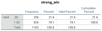
Image 1 – Frequency of dependent variable
Our initial attempts to build a predictive model for this analysis showed similar results in both decision trees and knn methodologies. In the case of decision tree, we varied the minimum number of observations in the parent and child nodes as well as the minimum improvement criteria. The best model achieved in decision tree was choosing a maximum tree depth of 5, minimum cases of 10 and 5 for parent and child respectively and a minimum change in improvement of 0.003; this tree has 6 nodes 4 of which are terminal nodes and a depth of 2.
The validation results of this model gave us a 78% accuracy, 99.6% precision in wins but 2.3% in losing games which is quite unreasonable, thus this model is not better than the just random assignment of predicting the strong team wins in all cases.The results were similar for the nearest neighbor algorithm, which achieved an accuracy rate of 75.5% and again a very low precision for lost games.
In order to improve the model’s precision we decided to undersample the dominating class of win = 1 so we could train the model with a more balanced distribution. To do this, we randomly selected 50% of the observations and then selected all rows with the minority class but only the ones selected randomly from the win rows. After performing this sampling selection, the algorithms improved significantly in terms of precision but then we also tried removing the overall difference variable from the models because there might me some multicollinearity because this should be a calculated field from the rest of the statistics. This last change improved precision even further.
The final decision tree was grown using a maximum depth of 10, minimum number of cases of 10 and 5 for parent and child respectively and a GINI minimum improvement in purity of 0.003. The precision increased drastically in losing games to 33.6%, maintaining the winning precision and by only dropping 5 points in the overall accuracy to reach 73.1%. This tree has 35 nodes 18 of which are terminal. Also when performing predictions for the entire data set we can see the the accuracy rate is actually better because there are more win observations for a final rate of 79%. Image 2 is a confusion matrix built over the predicted value and the real value in the entire dataset.
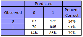 Image 2 – Final decision tree confusion matrix
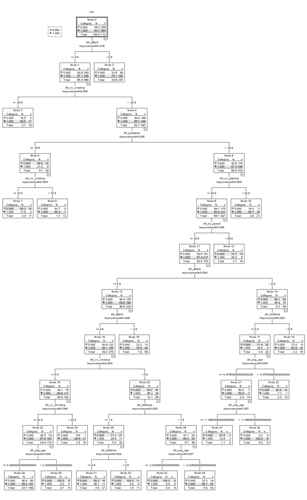
Image 3 – Final Decision tree
As we can see from image 3 the most important predictors are difference in attack, chance creation crossing, passing, speed, overall pressure, defense and midfield.
Conclusions
We conclude by selecting the decision tree with undersampling as our best model given the dataset. In general, sports outcome are difficult to predict so an accuracy of around 80% is reasonably acceptable. To explore in future analysis,given the amount of numerical variables, we think a logistic regression model might show better results. However, it was not possible to include this in the scope of our study.
Given the final model, we carried out predictions for the 2018 World Cup to be held in Russia this summer. To do this, we calculated winning odds for the round robin first, then for each team we averaged the probability of winning their three matches and assigned first and second of group to the ones with the highest and second highest probabilities respectively. In the cases where stats are not available, we used the min of each stat for the latest date since this are teams that have never been top 50 in FIFA ranking who are expected to underperform against the other teams. Calculated probabilities are shown in Image 4.
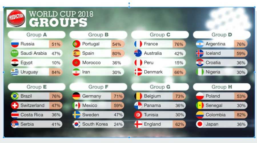
Image 4 – Predictions for 2018 World Cup groups
Given the matchups by the round robin prediction the teams that are most likely to reach the finals are Germany by one side with Spain or Germany on the other, if Brazil is to face Spain the model predicts Spain as the champion, but Brazil would beat Germany in a hypothetical final match.
Image 5 shows the predicted draw for the knockout phase along with the probability of reaching the spot they’re placed in. This was calculated by multiplying the probability of winning to the probability of reaching the round recursively all the way through the final round.
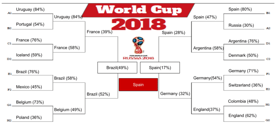
Image 5 – Predictions for 2018 World Cup
Future work can be done by trying a logistic regression model, given the amount of numeric variables we consider results can be further improved with a regression algorithm, another consideration could be to give weight to the wins or losses, because it is not the same to win by a one goal difference than to a three goal differences, considering this might help create a better model. Also to consider for future approaches is to look for stats for more countries or maybe use more updated stats son instead of every six months use every month or so.